Note
Go to the end to download the full example code.
Temporal Biases for Ordinary DSS.#
This example demonstrates DSS for extracting temporally structured signals: autocorrelated components, slow drifts, and smooth waveforms.
These ordinary-DSS bias operators do not perform lag-space TimeShiftDSS;
see the dedicated TimeShiftDSS guide for that repeated-trial FIR estimator.
We cover both linear biases (LagAverageBias, SmoothingBias) and nonlinear denoisers (DCTDenoiser, TemporalSmoothnessDenoiser).
The examples move from synthetic slow drifts to lag-averaging and smoothing biases, then to DCT-based iterative denoising and a real EEG slow-potential example.
- Authors: Sina Esmaeili (sina.esmaeili@umontreal.ca)
Hamza Abdelhedi (hamza.abdelhedi@umontreal.ca)
Imports#
import matplotlib.pyplot as plt
import mne
import numpy as np
from scipy import signal

from mne_denoise.dss import DSS, IterativeDSS
from mne_denoise.dss.denoisers import (
    DCTDenoiser,
    LagAverageBias,
    SmoothingBias,
)
from mne_denoise.dss.variants import smooth_dss
from mne_denoise.viz import (
    plot_channel_time_course_comparison,
    plot_component_summary,
    plot_psd_comparison,
)
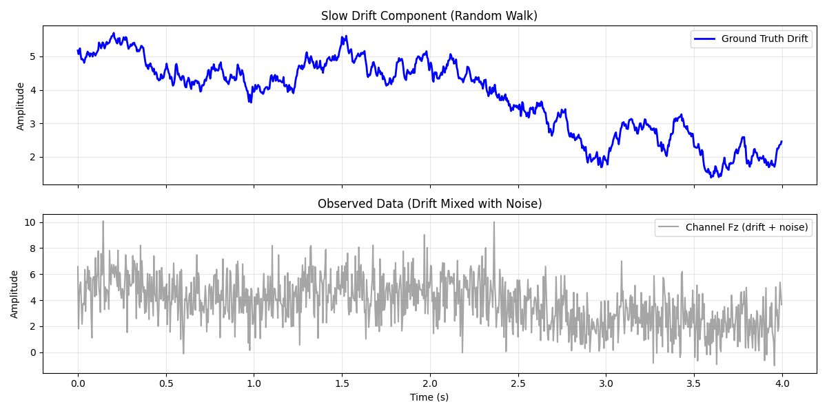
Part 0: Synthetic Slow Drift (Random Walk)#
Simulate slow cortical potentials: random walk + white noise
print("--- Part 0: Synthetic Slow Drift ---")

rng = np.random.default_rng(42)
sfreq = 250  # Hz
n_seconds = 30
n_times = n_seconds * sfreq
n_channels = 16
times = np.arange(n_times) / sfreq

# 1. Slow Drift (Random Walk - integrates white noise)
drift_seed = rng.normal(0, 0.05, n_times)
drift = np.cumsum(drift_seed)  # Random walk
drift = signal.detrend(drift)  # Remove DC
drift *= 2.0  # Scale

# 2. Fast Noise (White)
noise = rng.normal(0, 1.5, (n_channels, n_times))

# 3. Mix: First 4 channels get the drift
data = noise.copy()
data[:4] += drift * np.array([[1.0], [0.8], [0.6], [0.4]])

print(f"Simulated {n_channels} ch × {n_seconds}s with slow drift in first 4 channels")

# Create MNE Raw with montage
ch_names = [
    "Fz",
    "F3",
    "F4",
    "Cz",
    "C3",
    "C4",
    "Pz",
    "P3",
    "P4",
    "Oz",
    "O1",
    "O2",
    "Fp1",
    "Fp2",
    "T7",
    "T8",
]
info_sim = mne.create_info(ch_names, sfreq, "eeg")
montage = mne.channels.make_standard_montage("standard_1020")
info_sim.set_montage(montage)
raw_sim = mne.io.RawArray(data, info_sim)

# Visualize time series
fig, axes = plt.subplots(2, 1, figsize=(12, 6), sharex=True)
t_plot = times[:1000]  # First 4 seconds

axes[0].plot(t_plot, drift[:1000], "b", linewidth=2, label="Ground Truth Drift")
axes[0].set_title("Slow Drift Component (Random Walk)")
axes[0].set_ylabel("Amplitude")
axes[0].legend()
axes[0].grid(True, alpha=0.3)

axes[1].plot(
    t_plot, data[0, :1000], "gray", alpha=0.7, label="Channel Fz (drift + noise)"
)
axes[1].set_title("Observed Data (Drift Mixed with Noise)")
axes[1].set_xlabel("Time (s)")
axes[1].set_ylabel("Amplitude")
axes[1].legend()
axes[1].grid(True, alpha=0.3)

plt.tight_layout()
plt.show()
--- Part 0: Synthetic Slow Drift ---
Simulated 16 ch × 30s with slow drift in first 4 channels
Creating RawArray with float64 data, n_channels=16, n_times=7500
    Range : 0 ... 7499 =      0.000 ...    29.996 secs
Ready.
Part 1: Lag-averaging bias#
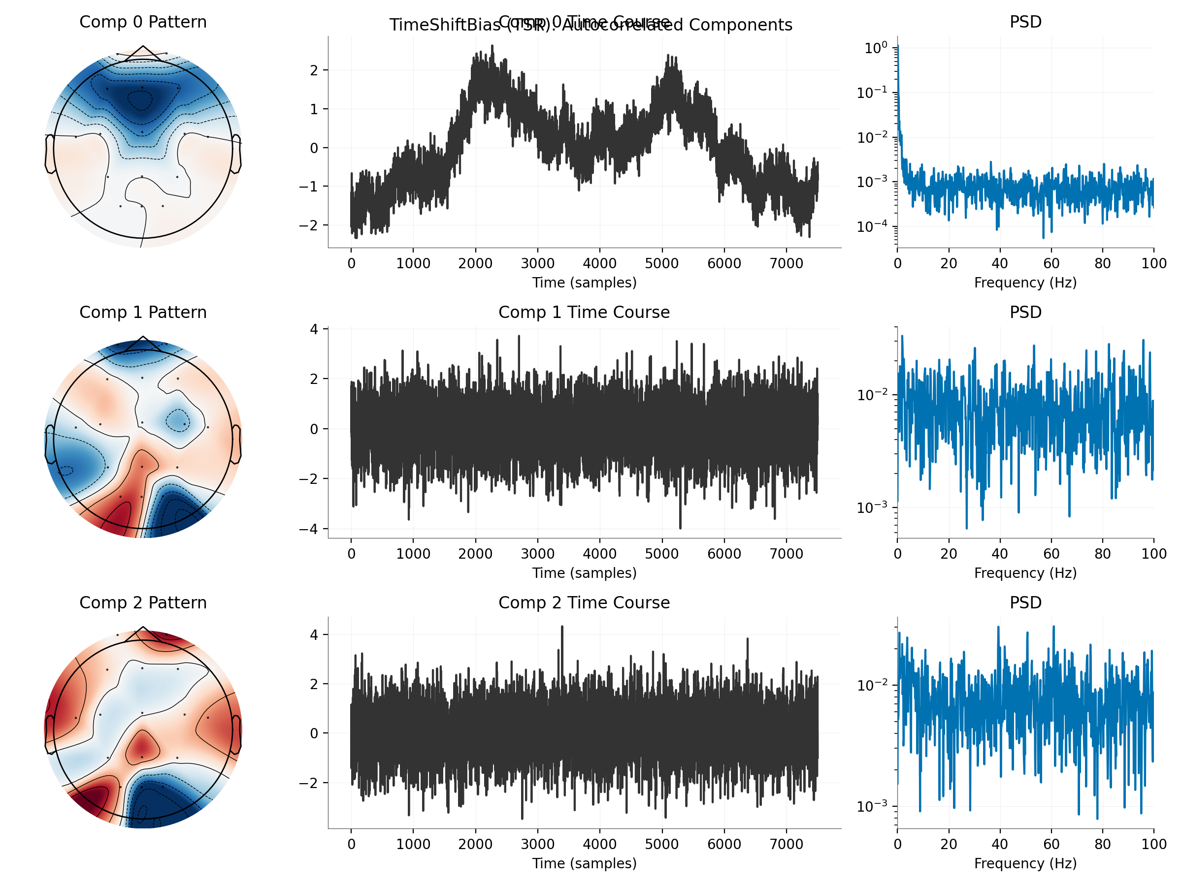
Lag averaging emphasizes components that remain similar across time lags.
print("\n--- Part 1: Lag Averaging ---")

# Explicit lag-averaging bias
bias_tsr = LagAverageBias(lags=10, weighting="uniform")
dss_tsr_manual = DSS(n_components=5, bias=bias_tsr)
dss_tsr_manual.fit(raw_sim)

print(f"Manual DSS Eigenvalues: {dss_tsr_manual.eigenvalues_[:5]}")

# Visualize the explicit DSS-plus-bias configuration
plot_component_summary(
    dss_tsr_manual,
    data=raw_sim,
    info=raw_sim.info,
    picks=np.arange(len(raw_sim.ch_names)),
    n_components=3,
    show=False,
)
plt.gcf().suptitle("LagAverageBias: Temporally Smooth Components")
plt.show()
--- Part 1: Lag Averaging ---
Manual DSS Eigenvalues: [0.90540147 0.1162555  0.11485271 0.11248996 0.11043523]
Compare first component with ground truth
sources_tsr = dss_tsr_manual.transform(raw_sim)
comp0_tsr = sources_tsr[0]

# Flip if negatively correlated
if np.corrcoef(comp0_tsr, drift)[0, 1] < 0:
    comp0_tsr *= -1

corr_tsr = np.corrcoef(comp0_tsr, drift)[0, 1]
print(f"\nCorrelation with ground truth drift: {corr_tsr:.3f}")

# Plot comparison
plt.figure(figsize=(12, 5))
t_zoom = times[:2000]  # First 8 seconds
plt.plot(t_zoom, drift[:2000], "b", linewidth=2, label="Ground Truth Drift", alpha=0.7)
plt.plot(
    t_zoom,
    comp0_tsr[:2000] * (np.std(drift) / np.std(comp0_tsr)),
    "r",
    linewidth=1.5,
    label=f"Lag-average component 0 (r={corr_tsr:.3f})",
    alpha=0.8,
)
plt.xlabel("Time (s)")
plt.ylabel("Amplitude (scaled)")
plt.title("Lag Averaging: Extracted Slow Drift")
plt.legend()
plt.grid(True, alpha=0.3)
plt.tight_layout()
plt.show()
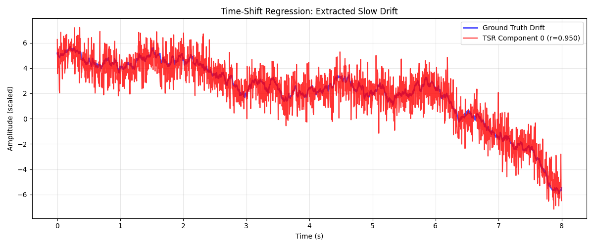
Correlation with ground truth drift: 0.950
Part 2: Temporal Smoothing (SmoothingBias)#
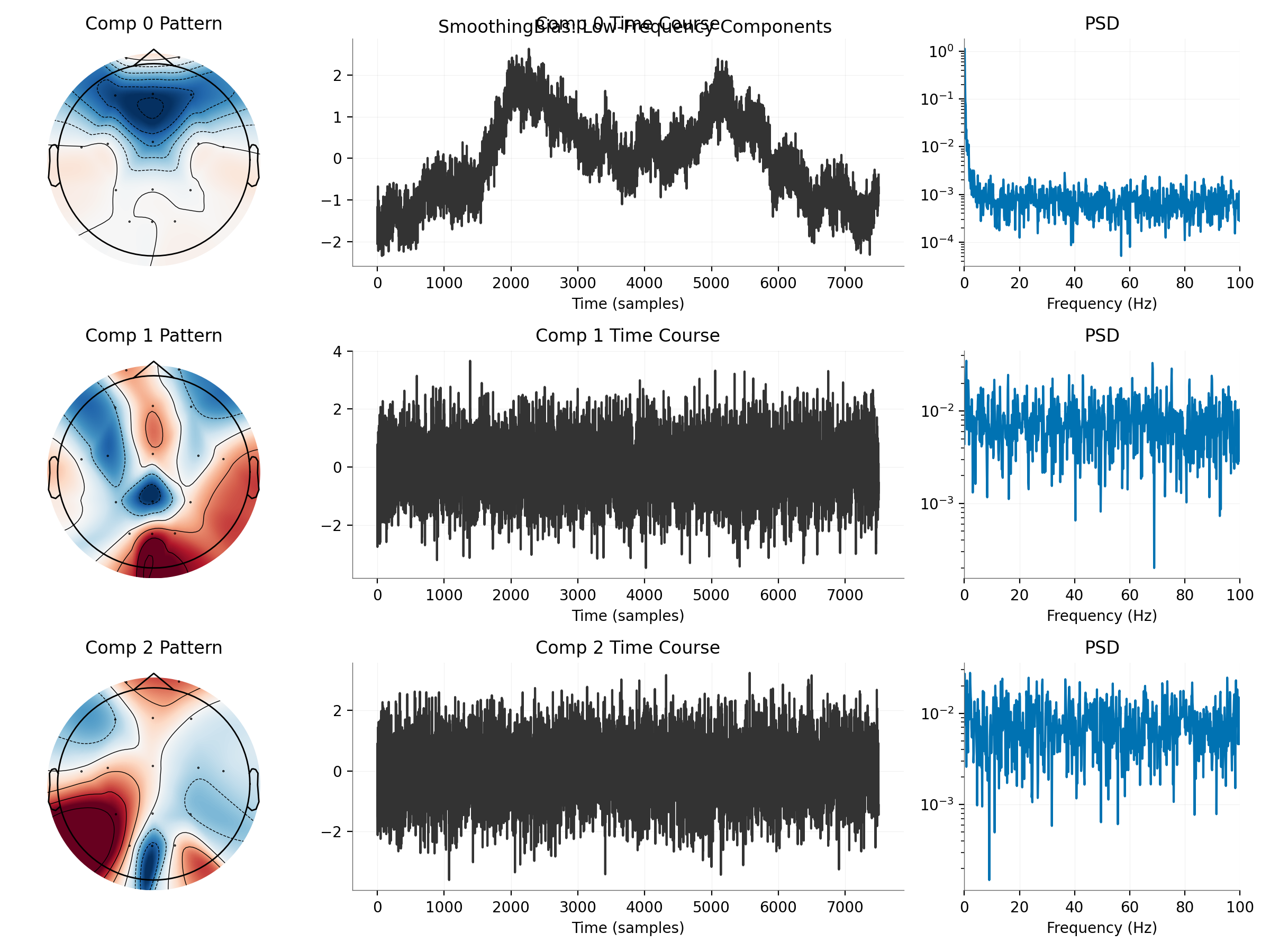
Emphasizes low-frequency temporal structure via smoothing
print("\n--- Part 2: Temporal Smoothing ---")

# Manual SmoothingBias
bias_smooth = SmoothingBias(window=50)  # 50 samples = 200ms at 250Hz
dss_smooth_manual = DSS(n_components=5, bias=bias_smooth)
dss_smooth_manual.fit(raw_sim)

print(f"Manual Smoothing Eigenvalues: {dss_smooth_manual.eigenvalues_[:5]}")

# Wrapper
dss_smooth_wrapper = smooth_dss(window=50, n_components=5)
dss_smooth_wrapper.fit(raw_sim)

print(f"Wrapper Eigenvalues: {dss_smooth_wrapper.eigenvalues_[:5]}")

# Visualize
plot_component_summary(
    dss_smooth_manual,
    data=raw_sim,
    info=raw_sim.info,
    picks=np.arange(len(raw_sim.ch_names)),
    n_components=3,
    show=False,
)
plt.gcf().suptitle("SmoothingBias: Low-Frequency Components")
plt.show()

# Compare with ground truth
sources_smooth = dss_smooth_manual.transform(raw_sim)
comp0_smooth = sources_smooth[0]

if np.corrcoef(comp0_smooth, drift)[0, 1] < 0:
    comp0_smooth *= -1

corr_smooth = np.corrcoef(comp0_smooth, drift)[0, 1]
print(f"\nCorrelation with ground truth: {corr_smooth:.3f}")
--- Part 2: Temporal Smoothing ---
Manual Smoothing Eigenvalues: [0.90215465 0.03167286 0.03000326 0.026934   0.0242747 ]
Wrapper Eigenvalues: [0.90215465 0.03167286 0.03000326 0.026934   0.0242747 ]

Correlation with ground truth: 0.950
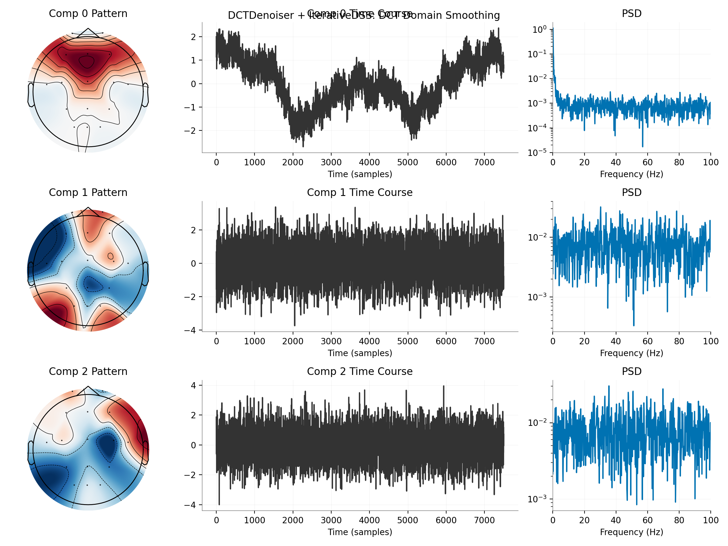
Part 3: DCT Denoiser (Nonlinear, IterativeDSS)#
DCT domain lowpass filtering for temporal smoothness
print("\n--- Part 3: DCT Denoiser + IterativeDSS ---")

# DCTDenoiser keeps first 30% of DCT coefficients (lowpass)
dct_denoiser = DCTDenoiser(cutoff_fraction=0.3)

# IterativeDSS with DCT denoising
idss_dct = IterativeDSS(denoiser=dct_denoiser, n_components=3, max_iter=5)

idss_dct.fit(raw_sim)

print("IterativeDSS (DCT) converged")

# Visualize
plot_component_summary(
    idss_dct,
    data=raw_sim,
    info=raw_sim.info,
    picks=np.arange(len(raw_sim.ch_names)),
    n_components=3,
    show=False,
)
plt.gcf().suptitle("DCTDenoiser + IterativeDSS: DCT Domain Smoothing")
plt.show()

# Compare with ground truth
sources_dct = idss_dct.transform(raw_sim)
comp0_dct = sources_dct[0]

if np.corrcoef(comp0_dct, drift)[0, 1] < 0:
    comp0_dct *= -1

corr_dct = np.corrcoef(comp0_dct, drift)[0, 1]
print(f"\nCorrelation with ground truth: {corr_dct:.3f}")
--- Part 3: DCT Denoiser + IterativeDSS ---
IterativeDSS (DCT) converged

Correlation with ground truth: 0.949
Compare All Methods#
Visualize how different temporal methods extract the drift
fig, axes = plt.subplots(4, 1, figsize=(14, 8), sharex=True)
t_compare = times[:2000]
scale = np.std(drift) / np.std(comp0_tsr)

axes[0].plot(t_compare, drift[:2000], "k", linewidth=2, label="Ground Truth")
axes[0].set_title("Ground Truth: Slow Drift (Random Walk)")
axes[0].set_ylabel("Amplitude")
axes[0].legend()
axes[0].grid(True, alpha=0.3)

axes[1].plot(
    t_compare,
    comp0_tsr[:2000] * scale,
    "r",
    label=f"Lag average (r={corr_tsr:.3f})",
)
axes[1].set_title("LagAverageBias")
axes[1].set_ylabel("Amplitude")
axes[1].legend()
axes[1].grid(True, alpha=0.3)

axes[2].plot(
    t_compare,
    comp0_smooth[:2000] * scale,
    "b",
    label=f"Smoothing (r={corr_smooth:.3f})",
)
axes[2].set_title("SmoothingBias (Moving Average)")
axes[2].set_ylabel("Amplitude")
axes[2].legend()
axes[2].grid(True, alpha=0.3)

axes[3].plot(t_compare, comp0_dct[:2000] * scale, "g", label=f"DCT (r={corr_dct:.3f})")
axes[3].set_title("DCTDenoiser (DCT Domain Lowpass)")
axes[3].set_ylabel("Amplitude")
axes[3].legend()
axes[3].grid(True, alpha=0.3)

plt.tight_layout()
plt.show()

print("\n--- All methods successfully extract the slow drift ---")
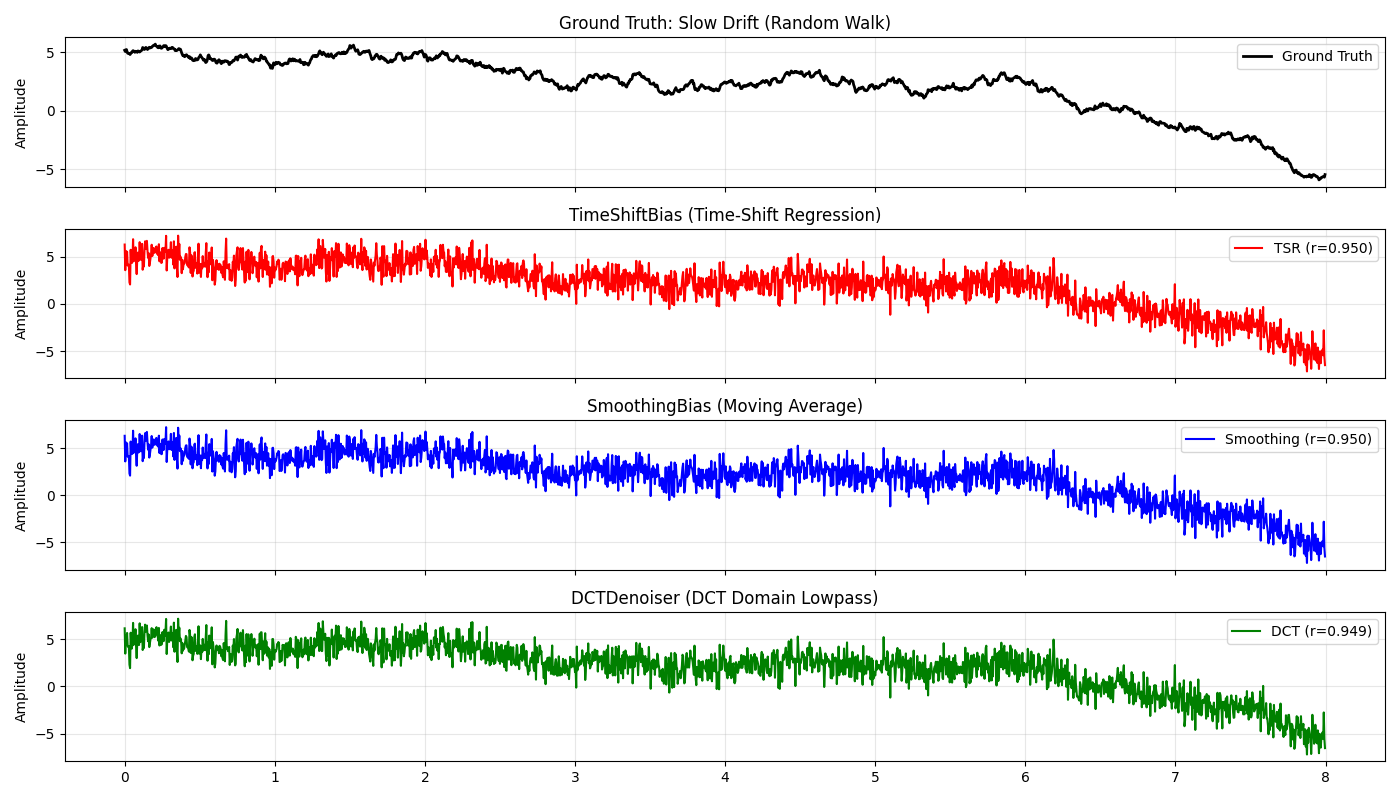
--- All methods successfully extract the slow drift ---
Part 4: Real EEG Data (Slow Cortical Potentials)#
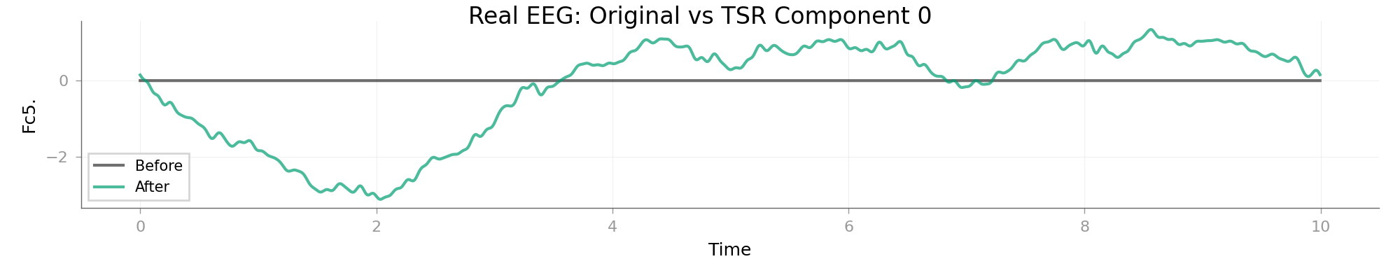
Apply lag-averaging DSS to real EEG for slow drift extraction
print("\n--- Part 4: Real EEG Data ---")

# Use eegbci dataset (resting state with eyes closed - has slow drifts)
from mne.datasets import eegbci

subject = 1
runs = [1]  # Baseline, eyes open
try:
    eegbci.load_data(subject, runs, update_path=True)
    raw_path = eegbci.load_data(subject, runs)[0]
except Exception as e:
    import sys

    print(f"Skipping EEGBCI example due to network error: {e}")
    sys.exit(0)

raw_eeg = mne.io.read_raw_edf(raw_path, preload=True, verbose=False)

# Add montage for topomap plotting
montage = mne.channels.make_standard_montage("standard_1005")
raw_eeg.set_montage(montage, on_missing="ignore", verbose=False)

raw_eeg.filter(0.1, 10, fir_design="firwin", verbose=False)  # Slow oscillations
raw_eeg.set_eeg_reference("average", projection=True, verbose=False)
raw_eeg.apply_proj()
raw_eeg.crop(0, 30)  # 30 seconds

print(f"EEG Data: {len(raw_eeg.ch_names)} channels, {raw_eeg.times[-1]:.1f}s")

# Apply lag-averaging DSS
dss_eeg_tsr = DSS(bias=LagAverageBias(lags=10), n_components=5)
dss_eeg_tsr.fit(raw_eeg)

print(f"\nLag-average eigenvalues: {dss_eeg_tsr.eigenvalues_[:5]}")

# Get sources for visualization
sources_eeg = dss_eeg_tsr.transform(raw_eeg)

# Create comparison plots using viz
raw_single = raw_eeg.copy().pick([0])  # First channel
comp_raw = mne.io.RawArray(
    sources_eeg[[0]], mne.create_info(1, raw_eeg.info["sfreq"], "eeg")
)

plot_channel_time_course_comparison(
    raw_single,
    comp_raw,
    picks=[0],
    times=raw_single.times,
    start=0,
    stop=int(10 * raw_single.info["sfreq"]),
    show=False,
)
plt.gcf().suptitle("Real EEG: Original vs Lag-Average Component 0")
plt.show()
--- Part 4: Real EEG Data ---
Created an SSP operator (subspace dimension = 1)
1 projection items activated
SSP projectors applied...
EEG Data: 64 channels, 30.0s

Lag-average eigenvalues: [0.99804042 0.99394146 0.99345606 0.99294188 0.99193759]
Creating RawArray with float64 data, n_channels=1, n_times=4801
    Range : 0 ... 4800 =      0.000 ...    30.000 secs
Ready.
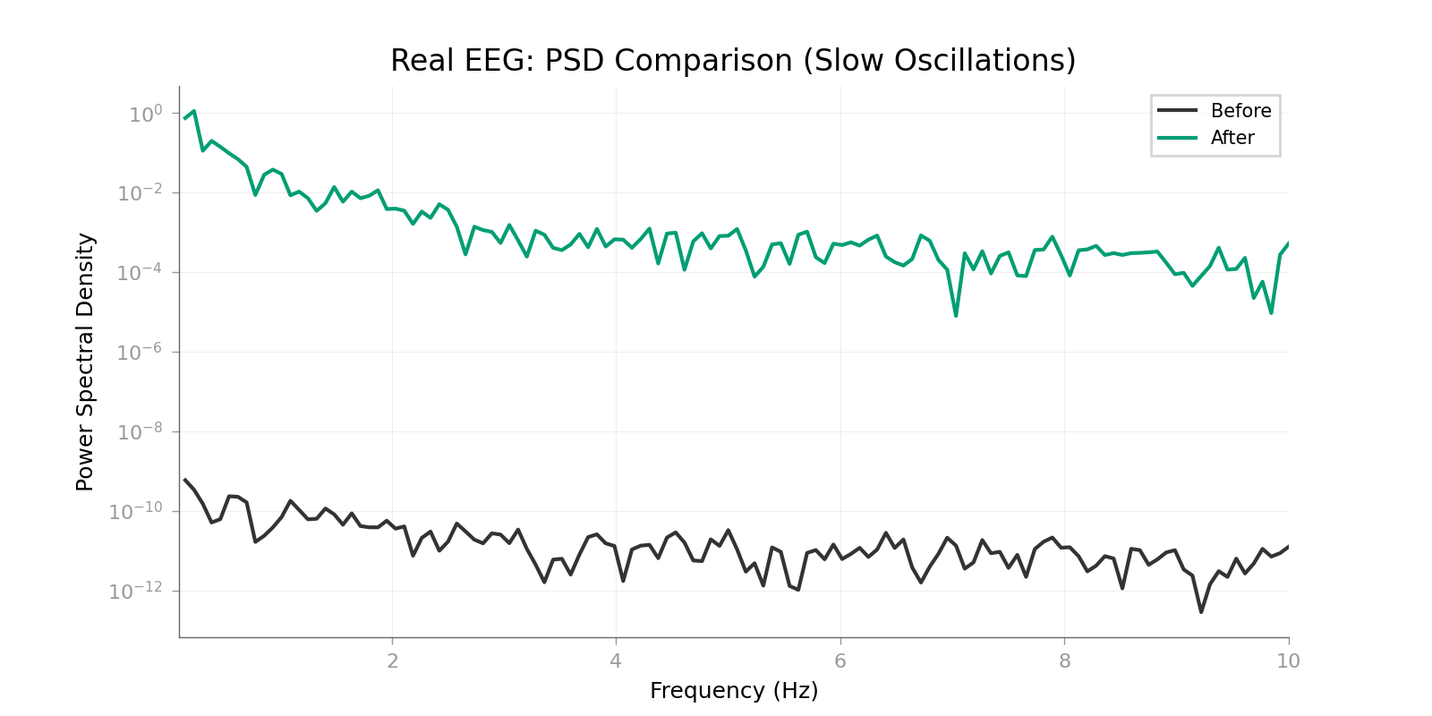
plot_psd_comparison(raw_single, comp_raw, fmin=0.1, fmax=10, show=False)
plt.gcf().axes[0].set_title("Real EEG: PSD Comparison (Slow Oscillations)")
plt.show()

print("\nLag-averaging DSS extracted slow cortical potentials from real EEG!")
Effective window size : 12.800 (s)
Effective window size : 12.800 (s)

Lag-averaging DSS extracted slow cortical potentials from real EEG!
Total running time of the script: (0 minutes 4.927 seconds)