ZapLine-plus: Adaptive Cleaning on Non-Stationary Noise.

This example follows the main steps of ZapLine-plus on a synthetic recording whose line noise changes in frequency, topography, and strength over time. The goal is to make the adaptive logic visible: frequency detection, segmentation, and chunk-wise cleaning.

Authors: Sina Esmaeili (sina.esmaeili@umontreal.ca)

import warnings

import matplotlib.pyplot as plt
import numpy as np
from matplotlib.gridspec import GridSpec
from scipy import signal

from mne_denoise.viz import plot_psd_comparison
from mne_denoise.zapline.adaptive import (
    check_artifact_presence,
    find_fine_peak,
    find_noise_freqs,
    segment_data,
)

# Suppress warnings for cleaner output
warnings.filterwarnings("ignore")

Paper Parameters

Match the paper’s recommended settings for comparison.

PAPER_PARAMS = {
    "minfreq": 17,  # Minimum search frequency (Hz)
    "maxfreq": 99,  # Maximum search frequency (Hz)
    "detectionWinsize": 6,  # Window size for detection (Hz)
    "coarseFreqDetectPowerDiff": 4,  # Threshold (10*log10 units, ~2.5x power)
    "noiseCompDetectSigma": 3.0,  # Initial sigma for outlier detection
    "minSigma": 2.5,  # Minimum sigma for adaptation
    "maxSigma": 4.0,  # Maximum sigma for adaptation (paper says 5, but 4 is safer)
    "minChunkLength": 30,  # Minimum chunk length (seconds)
    "segmentLength": 1,  # Segment length for covariance (seconds)
    "freqDetectMultFine": 2,  # Multiplier for fine detection threshold
    "detailedFreqBoundsUpper": [-0.05, 0.05],  # For "too weak" check
    "detailedFreqBoundsLower": [-0.4, 0.1],  # For "too strong" check
    "maxProportionAboveUpper": 0.005,
    "maxProportionBelowLower": 0.005,
}

Simulate Realistic Non-Stationary Data

Following the paper’s approach: line noise that varies in topography and strength over time.

def generate_nonstationary_data(
    sfreq=250,
    duration=180,  # 3 minutes
    n_ch=32,
    line_freq=50.0,
    seed=42,
):
    """Generate data with non-stationary line noise.

    The simulation has three regimes: a strong 50 Hz contamination with one
    topography from 0 to 60 seconds, a moderate 50.05 Hz contamination with a
    different topography from 60 to 120 seconds, and a final interval from 120
    to 180 seconds where noise appears only in bursts.
    """
    rng = np.random.RandomState(seed)
    n_times = int(duration * sfreq)
    times = np.arange(n_times) / sfreq

    # Background brain activity (pink noise-like)
    # Simulate 1/f spectrum using filtered noise
    brain = rng.randn(n_ch, n_times)
    # Low-pass to simulate neural activity spectrum
    sos = signal.butter(4, 40, btype="low", fs=sfreq, output="sos")
    brain = signal.sosfiltfilt(sos, brain, axis=1)
    brain = brain / np.std(brain) * 0.5  # Normalize

    # Define segment boundaries
    t1 = int(60 * sfreq)
    t2 = int(120 * sfreq)

    # Topography A: Frontal-like (strong on first channels)
    topo_a = np.exp(-np.linspace(0, 4, n_ch))
    topo_a /= np.linalg.norm(topo_a)

    # Topography B: Posterior-like (strong on last channels)
    topo_b = np.exp(-np.linspace(0, 4, n_ch)[::-1])
    topo_b /= np.linalg.norm(topo_b)

    # Topography C: Bipolar (alternating)
    topo_c = np.sin(np.linspace(0, 2 * np.pi, n_ch))
    topo_c /= np.linalg.norm(topo_c)

    # Initialize noise array
    noise = np.zeros((n_ch, n_times))

    # Chunk 1: Strong 50 Hz
    freq1 = line_freq
    ts1 = np.sin(2 * np.pi * freq1 * times[:t1])
    # Add harmonics (realistic line noise)
    ts1 += 0.3 * np.sin(2 * np.pi * 2 * freq1 * times[:t1])
    ts1 += 0.1 * np.sin(2 * np.pi * 3 * freq1 * times[:t1])
    noise[:, :t1] = np.outer(topo_a, ts1) * 3.0

    # Chunk 2: Moderate 50.05 Hz (frequency drift)
    freq2 = line_freq + 0.05
    ts2 = np.sin(2 * np.pi * freq2 * times[t1:t2])
    ts2 += 0.3 * np.sin(2 * np.pi * 2 * freq2 * times[t1:t2])
    noise[:, t1:t2] = np.outer(topo_b, ts2) * 1.5

    # Chunk 3: Bursts only
    # 10% of time has noise, 90% clean
    freq3 = line_freq - 0.05
    ts3 = np.sin(2 * np.pi * freq3 * times[t2:])
    burst_mask = np.zeros(n_times - t2)
    n_bursts = 5
    burst_len = int(sfreq * 2)  # 2s bursts
    for i in range(n_bursts):
        start = rng.randint(0, n_times - t2 - burst_len)
        burst_mask[start : start + burst_len] = 1.0
    noise[:, t2:] = np.outer(topo_c, ts3 * burst_mask) * 0.5

    data = brain + noise

    return (
        data,
        times,
        {
            "t1": t1,
            "t2": t2,
            "freq1": freq1,
            "freq2": freq2,
            "freq3": freq3,
            "topo_a": topo_a,
            "topo_b": topo_b,
            "topo_c": topo_c,
        },
    )

Generate Data

print("Generating non-stationary synthetic data...")
sfreq = 250
data, times, sim_info = generate_nonstationary_data(sfreq=sfreq)
n_ch, n_times = data.shape
duration = n_times / sfreq

print(f"  Shape: {n_ch} channels × {n_times} samples ({duration:.0f}s)")
print("  Noise structure:")
print(f"    0-60s:    {sim_info['freq1']} Hz, strong, frontal topography")
print(f"    60-120s:  {sim_info['freq2']} Hz, moderate, posterior topography")
print(f"    120-180s: {sim_info['freq3']} Hz, weak bursts, bipolar topography")

Generating non-stationary synthetic data...
  Shape: 32 channels × 45000 samples (180s)
  Noise structure:
    0-60s:    50.0 Hz, strong, frontal topography
    60-120s:  50.05 Hz, moderate, posterior topography
    120-180s: 49.95 Hz, weak bursts, bipolar topography

Step 1: Automatic Noise Frequency Detection

The paper uses a Welch PSD with Hanning window, then searches for peaks that exceed the “center power” (mean of flanks) by > 4 dB.

print("\n--- Step 1: Automatic Frequency Detection ---")
detected_freqs = find_noise_freqs(
    data,
    sfreq,
    fmin=PAPER_PARAMS["minfreq"],
    fmax=PAPER_PARAMS["maxfreq"],
    window_length=PAPER_PARAMS["detectionWinsize"],
    threshold_factor=PAPER_PARAMS["coarseFreqDetectPowerDiff"],
)
print(f"Detected noise frequencies: {detected_freqs}")

# Visualize detection
fig, ax = plt.subplots(figsize=(10, 4))
f, psd = signal.welch(data, fs=sfreq, nperseg=int(sfreq * 4), axis=-1)
psd_log = 10 * np.log10(np.clip(psd, 1e-20, None))
mean_psd = np.mean(psd_log, axis=0)

ax.plot(f, mean_psd, "k-", lw=1)
for freq in detected_freqs:
    ax.axvline(freq, color="r", ls="--", alpha=0.7, label=f"Detected: {freq:.1f} Hz")
ax.set_xlim(40, 70)
ax.set_xlabel("Frequency (Hz)")
ax.set_ylabel("Power (10*log10)")
ax.set_title("Automatic Noise Frequency Detection")
ax.legend()
plt.tight_layout()
plt.show()

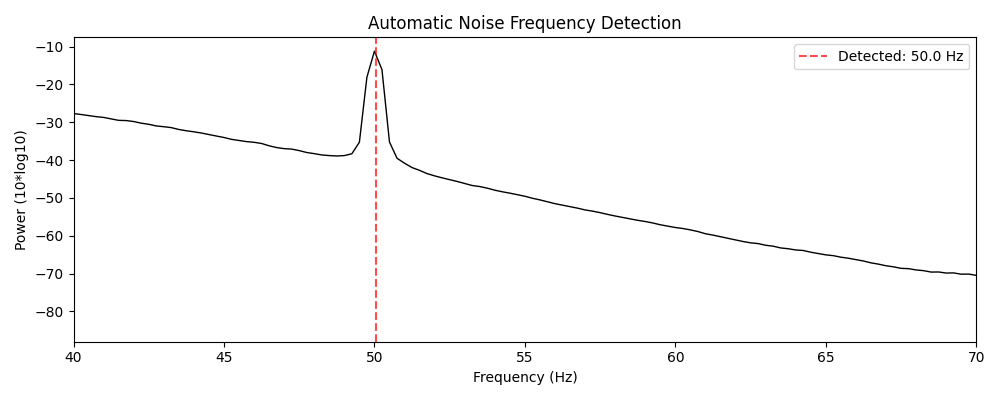
--- Step 1: Automatic Frequency Detection ---
Detected noise frequencies: [np.float64(50.048828125)]

Step 2: Adaptive Data Segmentation

Segment data based on covariance stationarity (changing noise topography). This is where ZapLine-plus differs most clearly from a single global fit.

print("\n--- Step 2: Adaptive Segmentation ---")
target_freq = detected_freqs[0] if detected_freqs else 50.0
segments = segment_data(
    data, sfreq, target_freq, min_chunk_len=PAPER_PARAMS["minChunkLength"]
)
print(f"Number of segments: {len(segments)}")
for i, (start, end) in enumerate(segments):
    print(
        f"  Segment {i + 1}: "
        f"{start / sfreq:.1f}s - {end / sfreq:.1f}s "
        f"({(end - start) / sfreq:.1f}s)"
    )

--- Step 2: Adaptive Segmentation ---
Number of segments: 3
  Segment 1: 0.0s - 60.0s (60.0s)
  Segment 2: 60.0s - 120.0s (60.0s)
  Segment 3: 120.0s - 180.0s (60.0s)

Step 3: Per-Segment Processing

For each segment we fine-tune the peak frequency, check whether an artifact is still present, and then run ZapLine with adaptive component selection.

print("\n--- Step 3: Per-Segment Processing ---")
segment_info = []
for i, (start, end) in enumerate(segments):
    chunk = data[:, start:end]

    # Fine-tune frequency
    fine_freq = find_fine_peak(chunk, sfreq, target_freq, search_width=0.1)

    # Check presence
    present = check_artifact_presence(chunk, sfreq, fine_freq)

    segment_info.append(
        {"start": start, "end": end, "fine_freq": fine_freq, "present": present}
    )

    status = "DETECTED" if present else "NOT DETECTED"
    print(f"  Segment {i + 1}: Fine freq = {fine_freq:.3f} Hz, Artifact {status}")

--- Step 3: Per-Segment Processing ---
  Segment 1: Fine freq = 50.000 Hz, Artifact DETECTED
  Segment 2: Fine freq = 50.050 Hz, Artifact DETECTED
  Segment 3: Fine freq = 49.950 Hz, Artifact DETECTED

Step 4: Apply Zapline-plus

Use the full pipeline with QA loop.

print("\n--- Step 4: Apply Zapline-plus ---")
from mne_denoise.zapline import ZapLine

# Configure adaptive ZapLine
zl = ZapLine(
    sfreq=sfreq,
    line_freq=target_freq,  # Use detected frequency or None
    adaptive=True,
    adaptive_params={
        "fmin": PAPER_PARAMS["minfreq"],
        "fmax": PAPER_PARAMS["maxfreq"],
        "n_remove_params": {
            "sigma": PAPER_PARAMS["noiseCompDetectSigma"],
            "min_remove": 1,
            "max_prop": 0.2,
        },
        "qa_params": {
            "max_sigma": PAPER_PARAMS["maxSigma"],
            "min_sigma": PAPER_PARAMS["minSigma"],
        },
    },
)

# Run Fit+Transform
data_clean = zl.fit_transform(data)
result = zl.adaptive_results_

print(f"Cleaning complete. Components removed: {result['n_removed']}")

--- Step 4: Apply Zapline-plus ---
Cleaning complete. Components removed: 4

Paper-Style Results Visualization

Use our reusable viz functions for quick overview, then custom plots.

# Quick overview using our viz functions
plot_psd_comparison(data, data_clean, sfreq=sfreq, line_freq=target_freq, show=True)

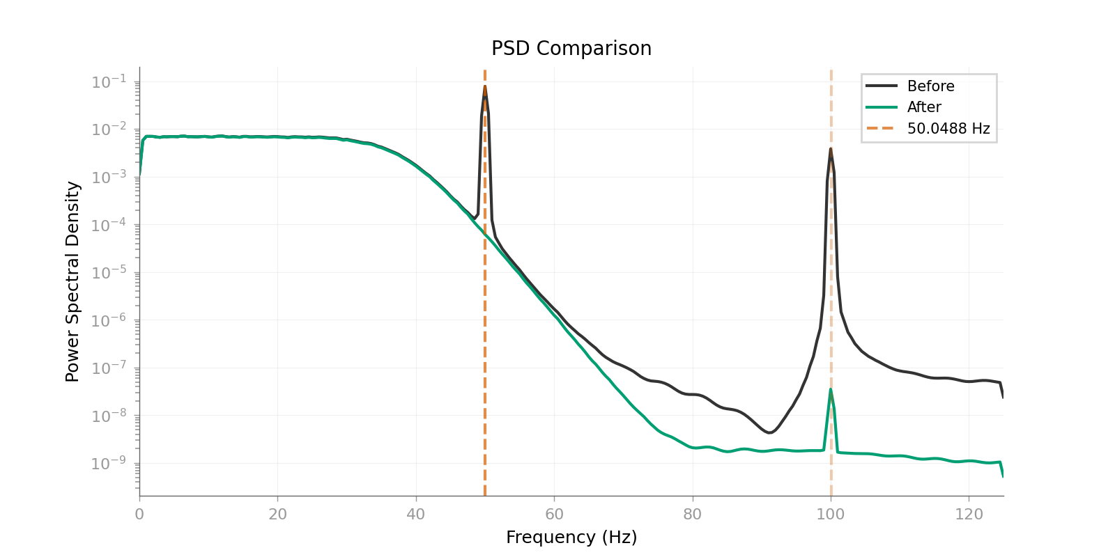
<Figure size 1600x800 with 1 Axes>

Detailed Adaptive Cleaning Figure

fig = plt.figure(figsize=(14, 10))
gs = GridSpec(3, 3, figure=fig, hspace=0.3, wspace=0.3)

# 1. Original vs Cleaned PSD (Full)
ax1 = fig.add_subplot(gs[0, :2])
f_orig, psd_orig = signal.welch(data, fs=sfreq, nperseg=int(sfreq * 4), axis=-1)
f_clean, psd_clean = signal.welch(data_clean, fs=sfreq, nperseg=int(sfreq * 4), axis=-1)

mean_orig = np.mean(10 * np.log10(np.clip(psd_orig, 1e-20, None)), axis=0)
mean_clean = np.mean(10 * np.log10(np.clip(psd_clean, 1e-20, None)), axis=0)

ax1.plot(f_orig, mean_orig, "k-", lw=1, label="Original")
ax1.plot(f_clean, mean_clean, "g-", lw=1.5, label="Cleaned")
ax1.set_xlim(0, 100)
ax1.set_xlabel("Frequency (Hz)")
ax1.set_ylabel("Power (dB)")
ax1.set_title("Power Spectral Density: Full Range")
ax1.legend()
ax1.grid(True, alpha=0.3)

# 2. Zoom on Noise Frequency
ax2 = fig.add_subplot(gs[0, 2])
ax2.plot(f_orig, mean_orig, "k-", lw=1, label="Original")
ax2.plot(f_clean, mean_clean, "g-", lw=1.5, label="Cleaned")
ax2.set_xlim(target_freq - 2, target_freq + 2)
ax2.set_xlabel("Frequency (Hz)")
ax2.set_title(f"Zoom: {target_freq:.1f} Hz ± 2 Hz")
ax2.legend()
ax2.grid(True, alpha=0.3)

# 3. Spectrogram (Original)
ax3 = fig.add_subplot(gs[1, 0])
f_spec, t_spec, Sxx = signal.spectrogram(
    data[0], fs=sfreq, nperseg=int(sfreq * 2), noverlap=int(sfreq)
)
im = ax3.pcolormesh(
    t_spec,
    f_spec,
    10 * np.log10(Sxx + 1e-20),
    shading="gouraud",
    cmap="viridis",
    vmin=-30,
    vmax=10,
)
ax3.set_ylim(45, 55)
ax3.set_xlabel("Time (s)")
ax3.set_ylabel("Frequency (Hz)")
ax3.set_title("Original (Ch 0)")
plt.colorbar(im, ax=ax3, label="dB")

# 4. Spectrogram (Cleaned)
ax4 = fig.add_subplot(gs[1, 1])
f_spec, t_spec, Sxx_clean = signal.spectrogram(
    data_clean[0], fs=sfreq, nperseg=int(sfreq * 2), noverlap=int(sfreq)
)
im = ax4.pcolormesh(
    t_spec,
    f_spec,
    10 * np.log10(Sxx_clean + 1e-20),
    shading="gouraud",
    cmap="viridis",
    vmin=-30,
    vmax=10,
)
ax4.set_ylim(45, 55)
ax4.set_xlabel("Time (s)")
ax4.set_ylabel("Frequency (Hz)")
ax4.set_title("Cleaned (Ch 0)")
plt.colorbar(im, ax=ax4, label="dB")

# 5. Spectrogram (Removed)
ax5 = fig.add_subplot(gs[1, 2])
removed = data - data_clean
f_spec, t_spec, Sxx_rem = signal.spectrogram(
    removed[0], fs=sfreq, nperseg=int(sfreq * 2), noverlap=int(sfreq)
)
im = ax5.pcolormesh(
    t_spec,
    f_spec,
    10 * np.log10(Sxx_rem + 1e-20),
    shading="gouraud",
    cmap="viridis",
    vmin=-30,
    vmax=10,
)
ax5.set_ylim(45, 55)
ax5.set_xlabel("Time (s)")
ax5.set_ylabel("Frequency (Hz)")
ax5.set_title("Removed (Ch 0)")
plt.colorbar(im, ax=ax5, label="dB")

# 6. Per-Segment Comparison
t1 = sim_info["t1"]
t2 = sim_info["t2"]

ax6 = fig.add_subplot(gs[2, 0])
f1, p1_o = signal.welch(data[:, :t1], fs=sfreq, nperseg=int(sfreq * 2), axis=-1)
f1, p1_c = signal.welch(data_clean[:, :t1], fs=sfreq, nperseg=int(sfreq * 2), axis=-1)
ax6.plot(f1, np.mean(10 * np.log10(p1_o + 1e-20), axis=0), "k-", label="Original")
ax6.plot(f1, np.mean(10 * np.log10(p1_c + 1e-20), axis=0), "g-", label="Cleaned")
ax6.set_xlim(45, 55)
ax6.set_title("Segment 1: 0-60s (Strong)")
ax6.set_xlabel("Frequency (Hz)")
ax6.set_ylabel("Power (dB)")
ax6.legend()
ax6.grid(True, alpha=0.3)

ax7 = fig.add_subplot(gs[2, 1])
f2, p2_o = signal.welch(data[:, t1:t2], fs=sfreq, nperseg=int(sfreq * 2), axis=-1)
f2, p2_c = signal.welch(data_clean[:, t1:t2], fs=sfreq, nperseg=int(sfreq * 2), axis=-1)
ax7.plot(f2, np.mean(10 * np.log10(p2_o + 1e-20), axis=0), "k-", label="Original")
ax7.plot(f2, np.mean(10 * np.log10(p2_c + 1e-20), axis=0), "g-", label="Cleaned")
ax7.set_xlim(45, 55)
ax7.set_title("Segment 2: 60-120s (Moderate)")
ax7.set_xlabel("Frequency (Hz)")
ax7.legend()
ax7.grid(True, alpha=0.3)

ax8 = fig.add_subplot(gs[2, 2])
f3, p3_o = signal.welch(data[:, t2:], fs=sfreq, nperseg=int(sfreq * 2), axis=-1)
f3, p3_c = signal.welch(data_clean[:, t2:], fs=sfreq, nperseg=int(sfreq * 2), axis=-1)
ax8.plot(f3, np.mean(10 * np.log10(p3_o + 1e-20), axis=0), "k-", label="Original")
ax8.plot(f3, np.mean(10 * np.log10(p3_c + 1e-20), axis=0), "g-", label="Cleaned")
ax8.set_xlim(45, 55)
ax8.set_title("Segment 3: 120-180s (Weak/Bursts)")
ax8.set_xlabel("Frequency (Hz)")
ax8.legend()
ax8.grid(True, alpha=0.3)

fig.suptitle("Zapline-plus Results: Non-Stationary Line Noise Removal", fontsize=14)
plt.tight_layout()
plt.show()

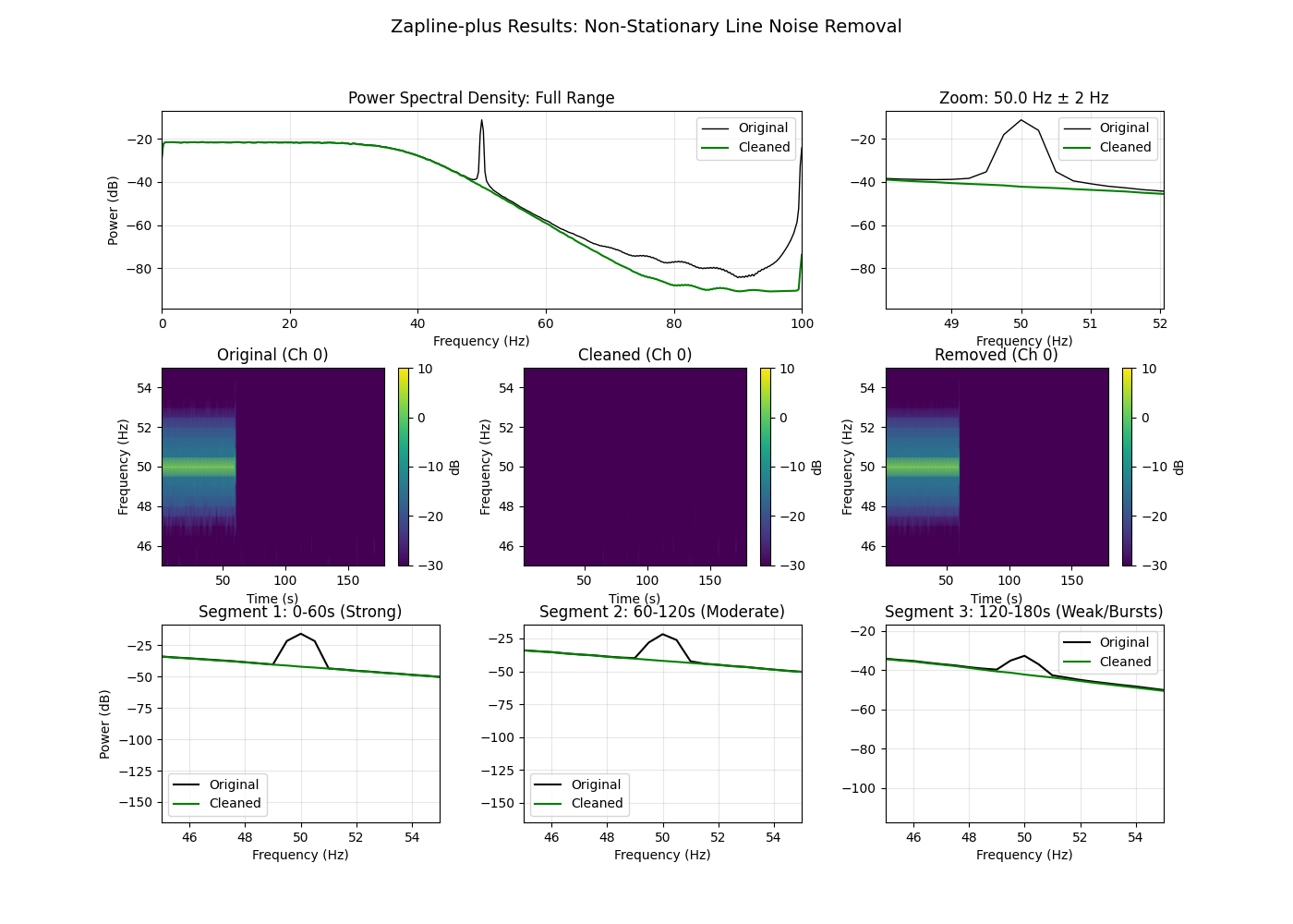
Quantitative Evaluation

Compute metrics similar to the paper.

print("\n--- Quantitative Evaluation ---")


def compute_noise_ratio(data_orig, data_clean, sfreq, noise_freq, win=0.5):
    """Compute ratio of power at noise freq to surroundings."""
    f, psd_o = signal.welch(data_orig, fs=sfreq, nperseg=int(sfreq * 2), axis=-1)
    f, psd_c = signal.welch(data_clean, fs=sfreq, nperseg=int(sfreq * 2), axis=-1)

    psd_o = np.mean(psd_o, axis=0)
    psd_c = np.mean(psd_c, axis=0)

    # Noise band
    noise_mask = (f > noise_freq - win) & (f < noise_freq + win)
    # Surroundings (flanks)
    surr_mask = ((f > noise_freq - 3) & (f < noise_freq - 1)) | (
        (f > noise_freq + 1) & (f < noise_freq + 3)
    )

    ratio_orig = np.mean(psd_o[noise_mask]) / np.mean(psd_o[surr_mask])
    ratio_clean = np.mean(psd_c[noise_mask]) / np.mean(psd_c[surr_mask])

    return ratio_orig, ratio_clean


# Overall
ratio_o, ratio_c = compute_noise_ratio(data, data_clean, sfreq, target_freq)
print(f"Noise/Surroundings Ratio: {ratio_o:.2f}x → {ratio_c:.2f}x (target ~1.0)")

# Per segment
ratio_o1, ratio_c1 = compute_noise_ratio(
    data[:, :t1], data_clean[:, :t1], sfreq, sim_info["freq1"]
)
ratio_o2, ratio_c2 = compute_noise_ratio(
    data[:, t1:t2], data_clean[:, t1:t2], sfreq, sim_info["freq2"]
)
ratio_o3, ratio_c3 = compute_noise_ratio(
    data[:, t2:], data_clean[:, t2:], sfreq, sim_info["freq3"]
)

print(f"  Segment 1 (Strong):   {ratio_o1:.2f}x → {ratio_c1:.2f}x")
print(f"  Segment 2 (Moderate): {ratio_o2:.2f}x → {ratio_c2:.2f}x")
print(f"  Segment 3 (Weak):     {ratio_o3:.2f}x → {ratio_c3:.2f}x")

# Power removed
total_power_orig = np.var(data)
total_power_clean = np.var(data_clean)
pct_removed = (1 - total_power_clean / total_power_orig) * 100
print(f"\nTotal Power Removed: {pct_removed:.2f}%")

print("\n[OK] Example complete!")

--- Quantitative Evaluation ---
Noise/Surroundings Ratio: 510.46x → 0.75x (target ~1.0)
  Segment 1 (Strong):   2162.88x → 0.74x
  Segment 2 (Moderate): 390.96x → 0.77x
  Segment 3 (Weak):     5.94x → 0.75x

Total Power Removed: 21.10%

[OK] Example complete!