ZapLine on MEG-like data with many co-equal noise components.

This example demonstrates the auto-mode fix from Issue #34. With high-channel-count MEG recordings (e.g., CTF 275-magnetometer systems), line noise couples into many sensors through different lead-field paths, producing several co-equal strong DSS components. The classic iterative_outlier_removal selector underdetects in this regime because no single eigenvalue stands out from the others; the new auto_select_components_robust falls back to a log-space knee detector that catches the cluster boundary.

The example uses synthetic data because the issue does not provide a public dataset, but the eigenvalue pattern reproduced here mirrors the one reported in mne-tools/mne-denoise#34.

Authors: Sina Esmaeili (sina.esmaeili@umontreal.ca)

Imports

import matplotlib.pyplot as plt
import numpy as np
from scipy import signal

from mne_denoise.dss.utils.selection import (
    auto_select_components_robust,
    detect_eigenvalue_knee,
    iterative_outlier_removal,
)
from mne_denoise.viz import plot_component_score_curve, plot_psd_comparison
from mne_denoise.zapline import ZapLine

Simulate a MEG-like recording

Three harmonics (50, 100, 150 Hz) couple into each of 64 channels with an independent phase and amplitude. This is a deliberately simple stand-in for the spatially heterogeneous line-noise pickup seen in real MEG.

rng = np.random.default_rng(34)
sfreq = 400
n_channels = 64
n_times = sfreq * 60  # 60 s
times = np.arange(n_times) / sfreq

line = np.zeros((n_channels, n_times))
for freq in (50.0, 100.0, 150.0):
    phases = rng.uniform(0, 2 * np.pi, n_channels)
    amps = rng.normal(1.0, 0.3, n_channels) * 5.0
    line += amps[:, None] * np.sin(2 * np.pi * freq * times[None, :] + phases[:, None])

# 1/f-ish brain background
background = rng.normal(0, 1, (n_channels, n_times))
sos = signal.butter(4, [1, 80], btype="bandpass", fs=sfreq, output="sos")
background = signal.sosfiltfilt(sos, background, axis=-1)
# Add a small 10 Hz alpha rhythm that we want to preserve
alpha = 0.3 * np.sin(2 * np.pi * 10.0 * times)
background += alpha[None, :]

data = background + line

Fit ZapLine in auto mode

zap = ZapLine(sfreq=sfreq, line_freq=50.0, n_remove="auto", n_harmonics=3)
zap.fit(data)
cleaned = zap.transform(data)

Inspect what each selection strategy returns

Before the fix, ZapLine called iterative_outlier_removal directly. On the user’s CTF data it returned 0 even though seven DSS eigenvalues clearly stood above the noise floor. The new auto_select_components_robust additionally runs detect_eigenvalue_knee and uses the larger of the two counts.

eigs = zap.eigenvalues_
n_outlier = iterative_outlier_removal(eigs, sigma=zap.threshold)
n_knee = detect_eigenvalue_knee(
    eigs, rel_floor=zap.knee_rel_floor, min_ratio=zap.knee_min_ratio
)
n_robust = auto_select_components_robust(
    eigs,
    sigma=zap.threshold,
    knee_rel_floor=zap.knee_rel_floor,
    knee_min_ratio=zap.knee_min_ratio,
)

print(f"iterative_outlier_removal -> {n_outlier}")
print(f"detect_eigenvalue_knee    -> {n_knee}")
print(f"auto_select_components_robust -> {n_robust}")
print(f"ZapLine n_removed_        -> {zap.n_removed_}")

iterative_outlier_removal -> 6
detect_eigenvalue_knee    -> 6
auto_select_components_robust -> 6
ZapLine n_removed_        -> 6

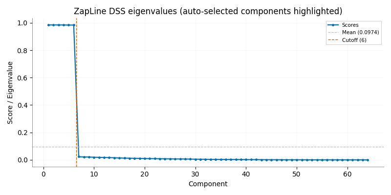
Visualize the eigenvalue spectrum

The knee marks the boundary between the line-noise cluster and the background floor.

fig, ax = plt.subplots(figsize=(8, 4))
plot_component_score_curve(zap, ax=ax, show=False)
ax.set_title("ZapLine DSS eigenvalues (auto-selected components highlighted)")
plt.tight_layout()
plt.show()

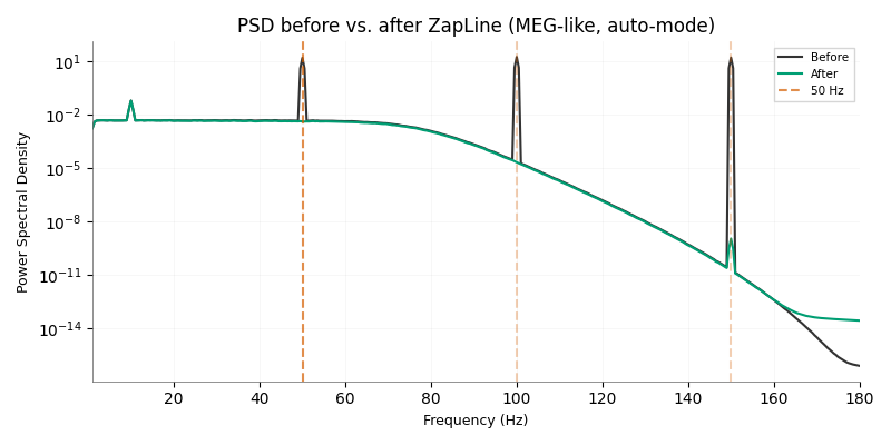
Confirm the cleaning worked

fig, ax = plt.subplots(figsize=(8, 4))
plot_psd_comparison(
    data,
    cleaned,
    sfreq=sfreq,
    line_freq=50.0,
    fmin=1,
    fmax=180,
    ax=ax,
    show=False,
)
ax.set_title("PSD before vs. after ZapLine (MEG-like, auto-mode)")
plt.tight_layout()
plt.show()

Workarounds for the rank-loss warning

Real CTF recordings can trip the rank-loss warning in mne_denoise.dss.linear.compute_dss() when channels with very different physical units are fit together, or when the baseline covariance spectrum spans many decades. Three options:

1. Pass normalize_input=True to mne_denoise.dss.linear.DSS when fitting DSS directly (ZapLine sets this to False by design).

2. Lower reg if the relative cutoff discards too many PCA dimensions.

3. Fit homogeneous channel types separately, e.g. use raw.copy().pick("mag") for CTF magnetometers instead of passing all channels at once.