ZapLine: Line Noise Removal Fundamentals.

This example introduces ZapLine on a controlled synthetic dataset. The goal is to show the basic workflow first on a simple 50 Hz contamination problem, then extend it to harmonics and more realistic multi-channel structure.

Reference:

de Cheveigné, A. (2020). ZapLine: A simple and effective method to remove power line artifacts. NeuroImage, 207, 116356.

Authors: Sina Esmaeili (sina.esmaeili@umontreal.ca)

Hamza Abdelhedi (hamza.abdelhedi@umontreal.ca)

Imports

import matplotlib.pyplot as plt
import numpy as np
from scipy import signal

from mne_denoise.viz import (
    plot_component_cleaning_summary,
    plot_component_score_curve,
    plot_psd_comparison,
)
from mne_denoise.zapline import ZapLine

Part 1: Synthetic Data

We create synthetic data with controllable line noise to demonstrate ZapLine’s effectiveness.

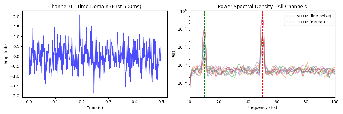
The data contains a 10 Hz neural signal we want to preserve, a 50 Hz line component we want to remove, and broadband noise.

print("Generating synthetic data with 50 Hz line noise...")

# Parameters
sfreq = 1000  # Sampling rate
duration = 5  # seconds
n_channels = 8
n_times = int(sfreq * duration)
t = np.arange(n_times) / sfreq

# Random state for reproducibility
rng = np.random.RandomState(42)

# Create mixing matrices for spatial structure
# Neural signal has one spatial pattern
neural_pattern = rng.randn(n_channels)
neural_pattern /= np.linalg.norm(neural_pattern)

# Line noise has a different spatial pattern
line_pattern = rng.randn(n_channels)
line_pattern /= np.linalg.norm(line_pattern)

# Generate source signals
neural_source = np.sin(2 * np.pi * 10 * t)  # 10 Hz neural
line_source = 2.0 * np.sin(2 * np.pi * 50 * t)  # 50 Hz line noise (strong)

# Mix to channels
data = np.zeros((n_channels, n_times))
for i in range(n_channels):
    data[i] = (
        neural_pattern[i] * neural_source
        + line_pattern[i] * line_source
        + rng.randn(n_times) * 0.5  # White noise
    )

print(f"Data shape: {data.shape}")
print("Signal: 10 Hz neural + 50 Hz line noise + white noise")

Generating synthetic data with 50 Hz line noise...
Data shape: (8, 5000)
Signal: 10 Hz neural + 50 Hz line noise + white noise

Visualize Original Data

Let’s look at the power spectral density (PSD) before cleaning.

fig, axes = plt.subplots(1, 2, figsize=(12, 4))

# Time domain
ax = axes[0]
ax.plot(t[:500], data[0, :500], "b-", alpha=0.7)
ax.set_xlabel("Time (s)")
ax.set_ylabel("Amplitude")
ax.set_title("Channel 0 - Time Domain (First 500ms)")

# Frequency domain
ax = axes[1]
freqs, psd = signal.welch(data, sfreq, nperseg=sfreq)
ax.semilogy(freqs, psd.T, alpha=0.5)
ax.axvline(50, color="r", linestyle="--", label="50 Hz (line noise)")
ax.axvline(10, color="g", linestyle="--", label="10 Hz (neural)")
ax.set_xlabel("Frequency (Hz)")
ax.set_ylabel("PSD")
ax.set_title("Power Spectral Density - All Channels")
ax.legend()
ax.set_xlim(0, 100)

plt.tight_layout()
plt.show()

Apply ZapLine

We use the ZapLine class to remove 50 Hz and its harmonics.

print("\nApplying ZapLine...")
# Instantiate ZapLine
est = ZapLine(
    line_freq=50,
    sfreq=sfreq,
    n_remove="auto",  # Automatically detect number of components
    threshold=2.5,  # Z-score threshold for auto-detection
)
est.fit(data)
cleaned = est.transform(data)

print(f"Components removed: {est.n_removed_}")
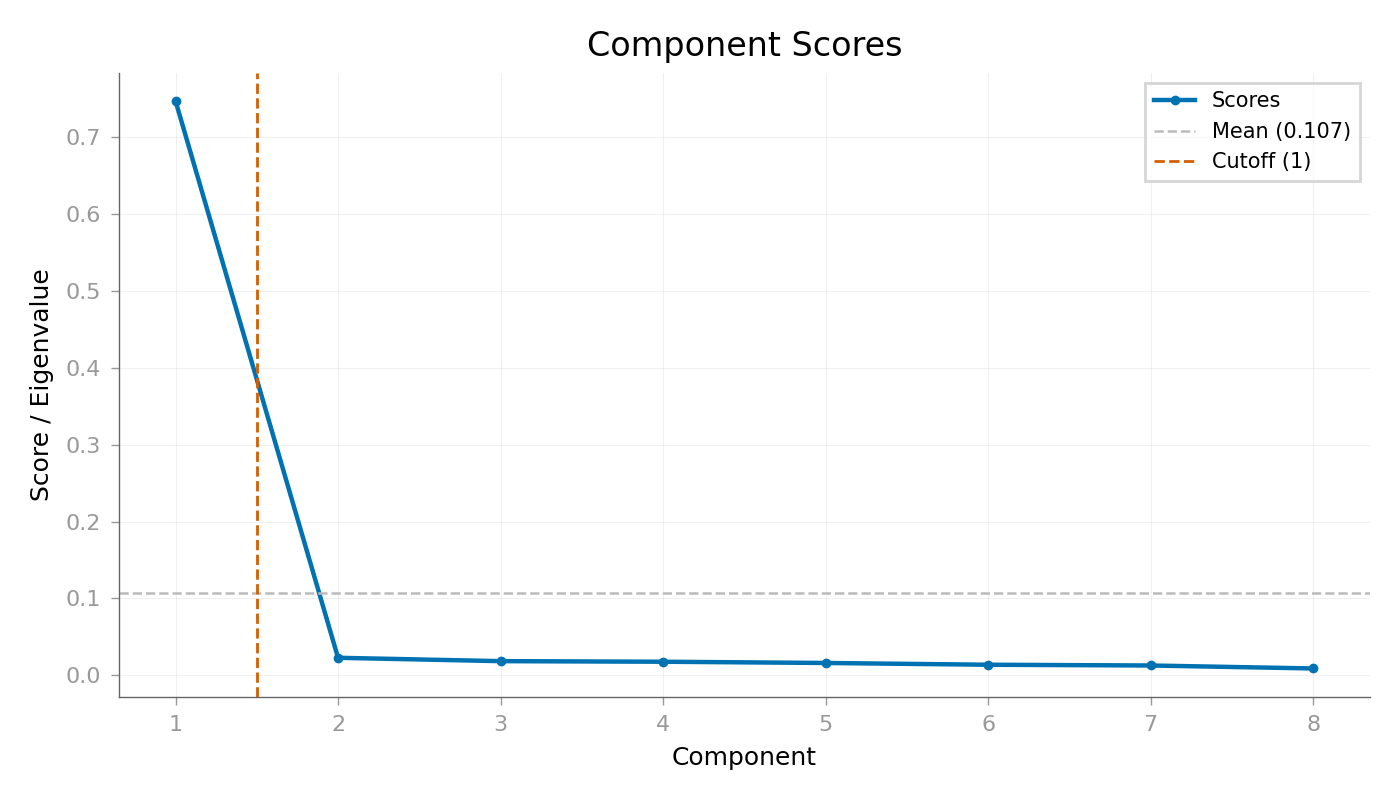
print(f"Component scores (eigenvalues): {est.eigenvalues_}")
print(f"Harmonics processed: {est.n_harmonics_}")

Applying ZapLine...
Components removed: 1
Component scores (eigenvalues): [0.74636042 0.02295699 0.0186003  0.01783306 0.01621905 0.01392562
 0.01294437 0.00908762]
Harmonics processed: 10

Compare Before/After

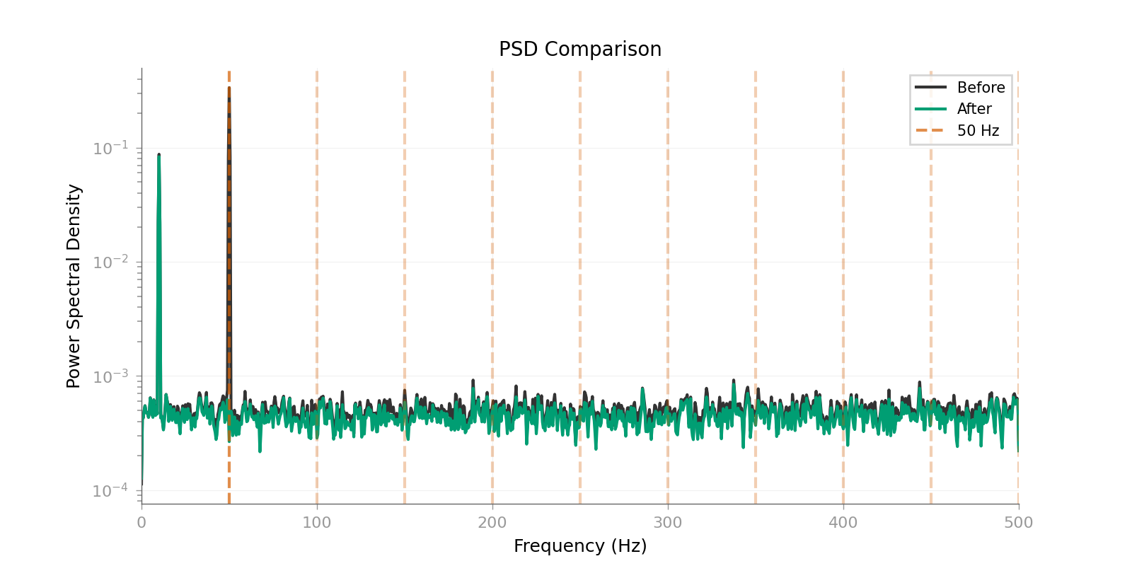
Let’s visualize the cleaning effect using the reusable viz function.

# Use plot_psd_comparison for a clean comparison
plot_psd_comparison(data, cleaned, sfreq=sfreq, line_freq=50, show=True)

<Figure size 1600x800 with 1 Axes>

Component Scores

View the DSS component scores to understand what was removed.

plot_component_score_curve(est, show=True)

<Figure size 1400x800 with 1 Axes>

Cleaning Summary

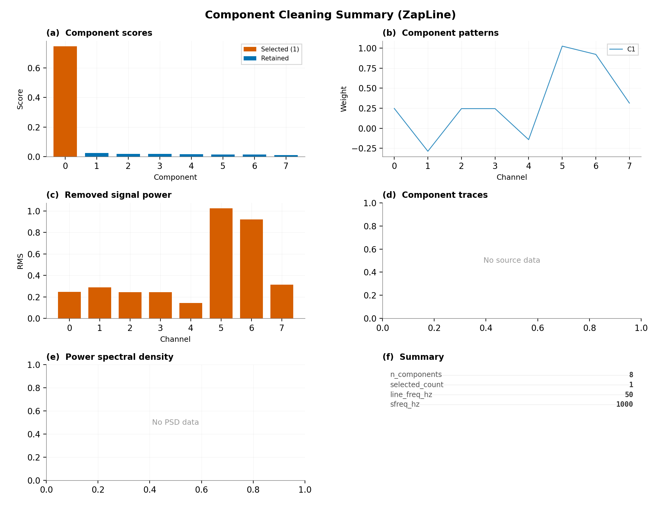
A comprehensive summary combining PSD, scores, and statistics.

plot_component_cleaning_summary(
    scores=getattr(est, "scores_", getattr(est, "eigenvalues_", None)),
    selected_count=getattr(est, "n_removed_", 0),
    patterns=getattr(est, "patterns_", None),
    removed=data - cleaned,
    sources=getattr(est, "sources_", None),
    sfreq=sfreq,
    line_freq=50,
    title="Component Cleaning Summary (ZapLine)",
    show=True,
)

/home/runner/work/mne-denoise/mne-denoise/mne_denoise/viz/theme.py:379: UserWarning: This figure includes Axes that are not compatible with tight_layout, so results might be incorrect.
  fig.tight_layout()

<Figure size 2200x1700 with 6 Axes>

Quantify Reduction

Measure the power reduction at 50 Hz.

idx_50 = np.argmin(np.abs(freqs - 50))
idx_10 = np.argmin(np.abs(freqs - 10))

_, psd_orig = signal.welch(data, sfreq, nperseg=sfreq)
_, psd_clean = signal.welch(cleaned, sfreq, nperseg=sfreq)

power_50_orig = np.mean(psd_orig[:, idx_50])
power_50_clean = np.mean(psd_clean[:, idx_50])
power_10_orig = np.mean(psd_orig[:, idx_10])
power_10_clean = np.mean(psd_clean[:, idx_10])

reduction_50_db = 10 * np.log10(power_50_orig / power_50_clean)
preservation_10 = power_10_clean / power_10_orig * 100

print("\n=== Results ===")
print(f"50 Hz power reduction: {reduction_50_db:.1f} dB")
print(f"10 Hz power preserved: {preservation_10:.1f}%")

=== Results ===
50 Hz power reduction: 26.1 dB
10 Hz power preserved: 94.9%

Part 2: Multi-Harmonic Removal

ZapLine can remove multiple harmonics of the line frequency. Let’s add harmonics to our synthetic data.

print("\n\nPart 2: Multi-Harmonic Line Noise")

# Add harmonics
line_source_harmonics = (
    2.0 * np.sin(2 * np.pi * 50 * t)  # 50 Hz
    + 1.0 * np.sin(2 * np.pi * 100 * t)  # 100 Hz (2nd harmonic)
    + 0.5 * np.sin(2 * np.pi * 150 * t)  # 150 Hz (3rd harmonic)
)

data_harmonics = np.zeros((n_channels, n_times))
for i in range(n_channels):
    data_harmonics[i] = (
        neural_pattern[i] * neural_source
        + line_pattern[i] * line_source_harmonics
        + rng.randn(n_times) * 0.5
    )

# Apply ZapLine
est_harmonics = ZapLine(
    line_freq=50,
    sfreq=sfreq,
    n_remove=1,
    n_harmonics=3,  # Explicitly request 3 harmonics
)
est_harmonics.fit(data_harmonics)
cleaned_harmonics = est_harmonics.transform(data_harmonics)

print(f"Harmonics processed: {est_harmonics.n_harmonics_}")

# Compare PSDs
fig, ax = plt.subplots(figsize=(10, 5))
freqs, psd_orig = signal.welch(data_harmonics, sfreq, nperseg=sfreq)
freqs, psd_clean = signal.welch(cleaned_harmonics, sfreq, nperseg=sfreq)

ax.semilogy(freqs, np.mean(psd_orig, axis=0), "b-", label="Original", alpha=0.7)
ax.semilogy(freqs, np.mean(psd_clean, axis=0), "g-", label="Cleaned")

for h in [50, 100, 150]:
    ax.axvline(h, color="r", linestyle="--", alpha=0.5)

ax.set_xlabel("Frequency (Hz)")
ax.set_ylabel("PSD")
ax.set_title("ZapLine Removes All Harmonics")
ax.legend()
ax.set_xlim(0, 200)
plt.show()

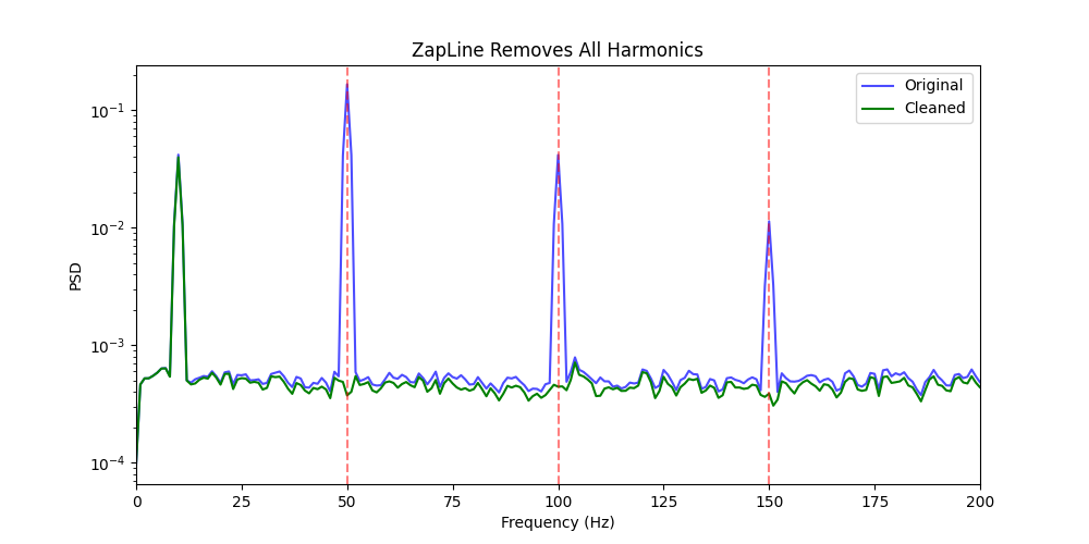
Part 2: Multi-Harmonic Line Noise
Harmonics processed: 3

Conclusion

ZapLine is effective because it targets spatial components that carry line noise, handles harmonics naturally, and can preserve neural structure even near the contaminated frequency. It can also choose the number of removed components automatically when that is more practical than fixing the value in advance.

The main parameters are line_freq for the mains frequency, n_remove for manual or automatic component selection, n_harmonics for harmonic coverage, and nkeep for optional PCA reduction on high-channel data.