Note
Go to the end to download the full example code.
Time-Frequency DSS: Spectrogram Masking.#
This example demonstrates DSS for extracting transient oscillatory bursts using time-frequency (TF) domain constraints via spectrogram masking.
We cover SpectrogramBias (linear) and SpectrogramDenoiser (nonlinear) for isolating activity that is sparse in the TF domain.
The examples move from synthetic spindle-like bursts to fixed-mask DSS, adaptive spectrogram denoising, and a real MEG gamma-burst example.
- Authors: Sina Esmaeili (sina.esmaeili@umontreal.ca)
Hamza Abdelhedi (hamza.abdelhedi@umontreal.ca)
Imports#
import matplotlib.pyplot as plt
import mne
import numpy as np
from mne.datasets import somato
from scipy import signal as sp_signal

from mne_denoise.dss import DSS, IterativeDSS
from mne_denoise.dss.denoisers import SpectrogramBias, SpectrogramDenoiser
from mne_denoise.viz import (
    plot_channel_time_course_comparison,
    plot_component_spectrogram,
    plot_component_summary,
    plot_signal_overlay,
    plot_spectrogram_comparison,
    plot_time_frequency_mask,
)
Part 0: Synthetic Transient Bursts (Sleep Spindles)#
Simulate 12 Hz spindle bursts embedded in noise
print("--- Part 0: Synthetic Spindle Bursts ---")

rng = np.random.default_rng(42)
sfreq = 250  # Hz
n_seconds = 10
n_times = n_seconds * sfreq
times = np.arange(n_times) / sfreq

# Background noise (broadband)
noise = rng.normal(0, 1.0, n_times)

# Spindle bursts at specific times
spindle_freq = 12.0  # Hz
envelope = np.zeros_like(times)

# Burst 1: 2-3 seconds
mask1 = (times >= 2) & (times < 3)
envelope[mask1] = np.hanning(mask1.sum())

# Burst 2: 7-8 seconds
mask2 = (times >= 7) & (times < 8)
envelope[mask2] = np.hanning(mask2.sum())

signal_spindle = envelope * np.sin(2 * np.pi * spindle_freq * times) * 3.0

# Mixed data
data_mixed = signal_spindle + noise

# Visualize
fig, axes = plt.subplots(3, 1, figsize=(14, 8), sharex=True)

axes[0].plot(times, signal_spindle, "b", linewidth=1.5, label="Clean Spindle")
axes[0].set_title("Ground Truth: 12 Hz Spindle Bursts")
axes[0].set_ylabel("Amplitude")
axes[0].legend()
axes[0].grid(True, alpha=0.3)

axes[1].plot(times, noise, "gray", alpha=0.7, label="Broadband Noise")
axes[1].set_title("Noise")
axes[1].set_ylabel("Amplitude")
axes[1].legend()
axes[1].grid(True, alpha=0.3)

axes[2].plot(times, data_mixed, "r", alpha=0.7, label="Mixed (Signal + Noise)")
axes[2].set_title("Observed Data")
axes[2].set_xlabel("Time (s)")
axes[2].set_ylabel("Amplitude")
axes[2].legend()
axes[2].grid(True, alpha=0.3)

plt.tight_layout()
plt.show()
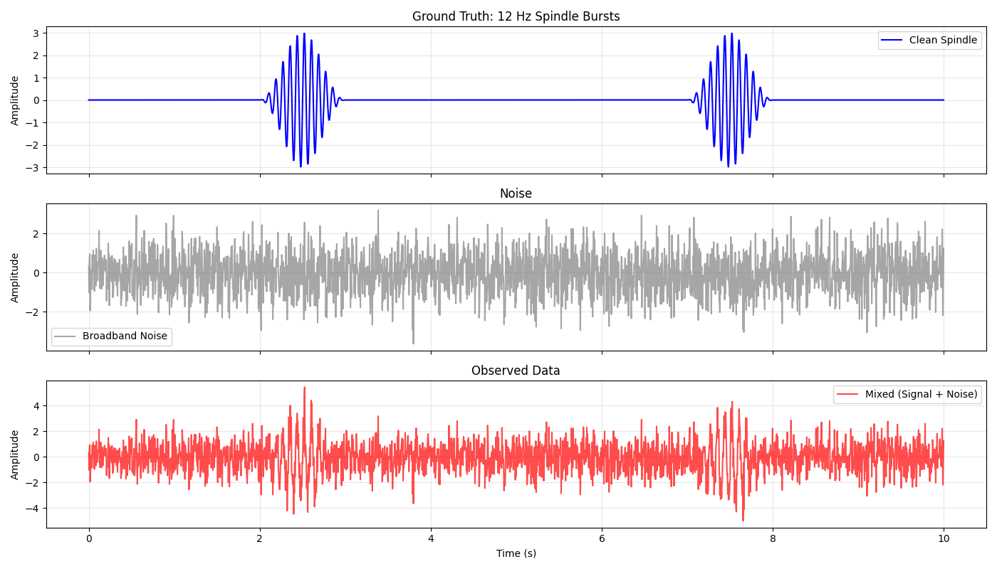
--- Part 0: Synthetic Spindle Bursts ---
Visualize Time-Frequency Representation#
Compute spectrogram to see bursts in TF domain
f, t, Sxx = sp_signal.spectrogram(data_mixed, fs=sfreq, nperseg=128, noverlap=96)

plt.figure(figsize=(12, 5))
plt.pcolormesh(t, f, 10 * np.log10(Sxx), shading="gouraud", cmap="viridis")
plt.colorbar(label="Power (dB)")
plt.ylabel("Frequency (Hz)")
plt.xlabel("Time (s)")
plt.title("Spectrogram: Spindle Bursts in Time-Frequency Domain")
plt.ylim(0, 30)
plt.axhline(spindle_freq, color="r", linestyle="--", alpha=0.7, label="12 Hz Spindle")
plt.legend()
plt.tight_layout()
plt.show()
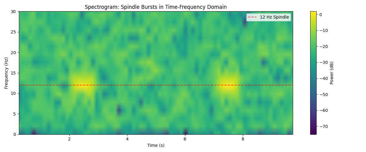
Part 1: SpectrogramBias with Fixed Mask#
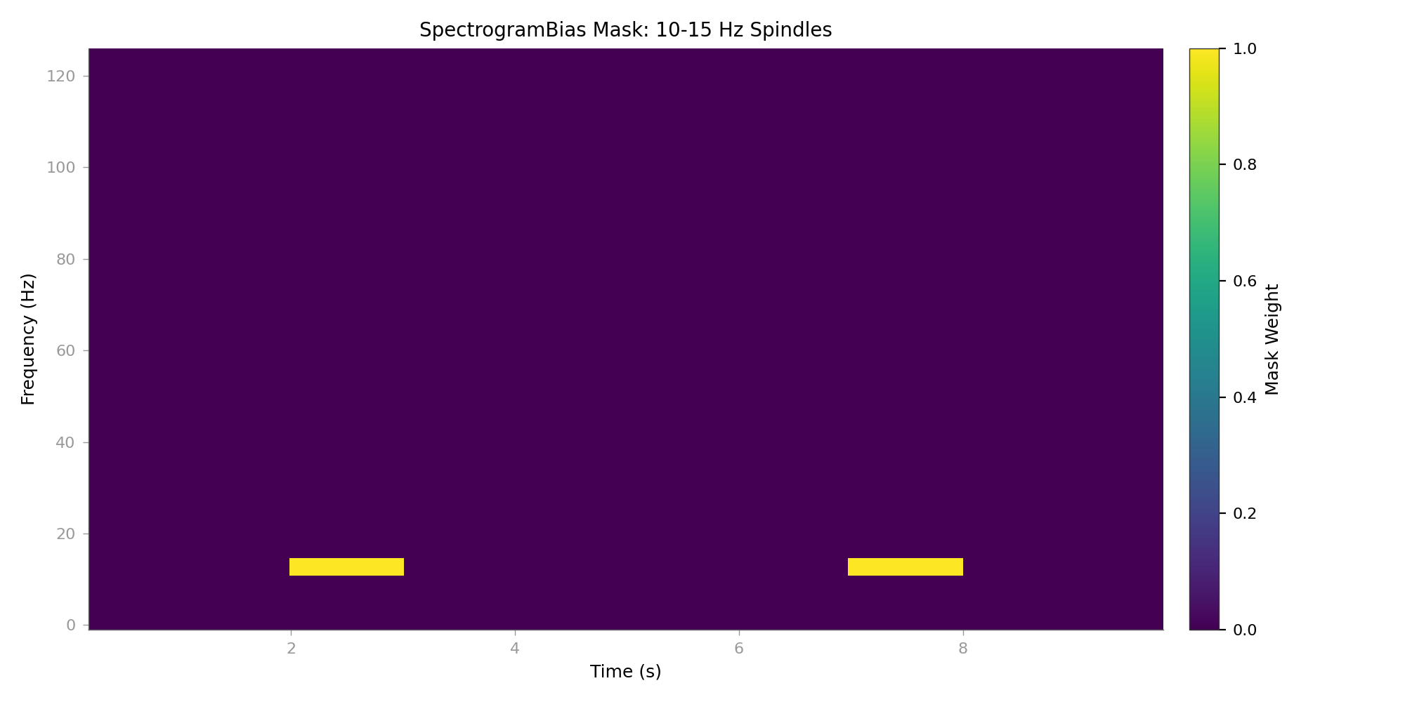
Define a TF mask to isolate burst regions
print("\n--- Part 1: Fixed TF Mask (SpectrogramBias) ---")

# Create manually defined TF mask for DSS
# Focus on 10-15 Hz range and burst time windows
nperseg = 128
noverlap = 96

# Get TF grid dimensions
_, t_grid, _ = sp_signal.spectrogram(
    data_mixed, fs=sfreq, nperseg=nperseg, noverlap=noverlap
)
n_freqs = nperseg // 2 + 1
n_times_tf = len(t_grid)

# Create mask: 1 where we expect spindles, 0 elsewhere
mask_fixed = np.zeros((n_freqs, n_times_tf))

# Define frequency band (10-15 Hz)
freq_axis = np.fft.rfftfreq(nperseg, 1 / sfreq)
freq_mask = (freq_axis >= 10) & (freq_axis <= 15)

# Define time windows for bursts
time_mask1 = (t_grid >= 2) & (t_grid < 3)
time_mask2 = (t_grid >= 7) & (t_grid < 8)

# Apply mask
mask_fixed[freq_mask[:, None] & (time_mask1 | time_mask2)] = 1.0

print(f"TF mask shape: {mask_fixed.shape}")
print(
    f"Masked points: {mask_fixed.sum()} / {mask_fixed.size} "
    f"({100 * mask_fixed.sum() / mask_fixed.size:.1f}%)"
)

# Visualize mask
plot_time_frequency_mask(
    mask_fixed,
    t_grid,
    freq_axis,
    title="SpectrogramBias Mask: 10-15 Hz Spindles",
    show=False,
)
plt.show()

# Apply SPectrogramBias with DSS
# For demonstration, create multi-channel data
n_channels = 8
data_multichan = np.tile(data_mixed, (n_channels, 1)) + rng.normal(
    0, 0.2, (n_channels, n_times)
)

# Create MNE Raw with montage for DSS
ch_names = ["Fz", "Cz", "Pz", "F3", "F4", "C3", "C4", "Oz"]
info = mne.create_info(ch_names, sfreq, "eeg")
montage = mne.channels.make_standard_montage("standard_1020")
info.set_montage(montage)
raw_spindle = mne.io.RawArray(data_multichan, info)

# Apply SpectrogramBias
bias_tf = SpectrogramBias(mask=mask_fixed, nperseg=nperseg, noverlap=noverlap)
dss_tf = DSS(n_components=3, bias=bias_tf)
dss_tf.fit(raw_spindle)

print(f"\nDSS Eigenvalues: {dss_tf.eigenvalues_[:3]}")

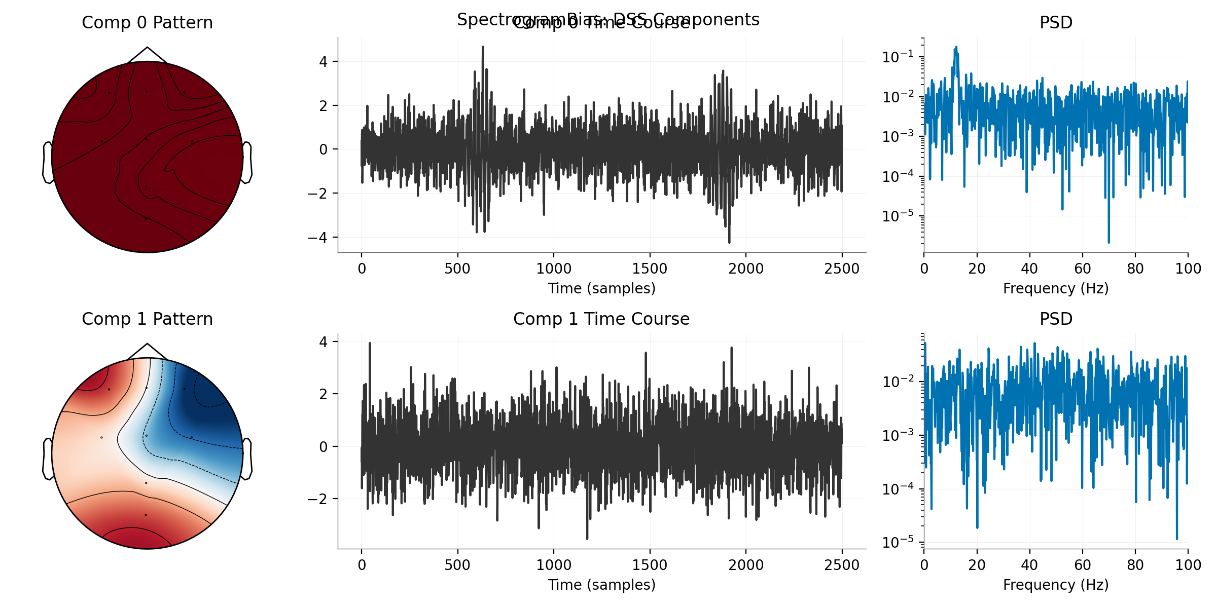
# Visualize DSS components
plot_component_summary(
    dss_tf,
    data=raw_spindle,
    info=raw_spindle.info,
    picks=np.arange(len(raw_spindle.ch_names)),
    n_components=2,
    show=False,
)
plt.gcf().suptitle("SpectrogramBias: DSS Components")
plt.show()

# Extract component
sources_tf = dss_tf.transform(raw_spindle)
comp0_tf = sources_tf[0]

# Compare with ground truth
if np.corrcoef(comp0_tf, signal_spindle)[0, 1] < 0:
    comp0_tf *= -1

corr_tf = np.corrcoef(comp0_tf, signal_spindle)[0, 1]
print(f"Correlation with ground truth: {corr_tf:.3f}")

# Spectrogram comparison
raw_orig = mne.io.RawArray(data_mixed[np.newaxis, :], mne.create_info(1, sfreq, "eeg"))
raw_comp = mne.io.RawArray(comp0_tf[np.newaxis, :], mne.create_info(1, sfreq, "eeg"))
--- Part 1: Fixed TF Mask (SpectrogramBias) ---
TF mask shape: (65, 75)
Masked points: 32.0 / 4875 (0.7%)
Creating RawArray with float64 data, n_channels=8, n_times=2500
    Range : 0 ... 2499 =      0.000 ...     9.996 secs
Ready.

DSS Eigenvalues: [0.18872036 0.01285285 0.00731457]
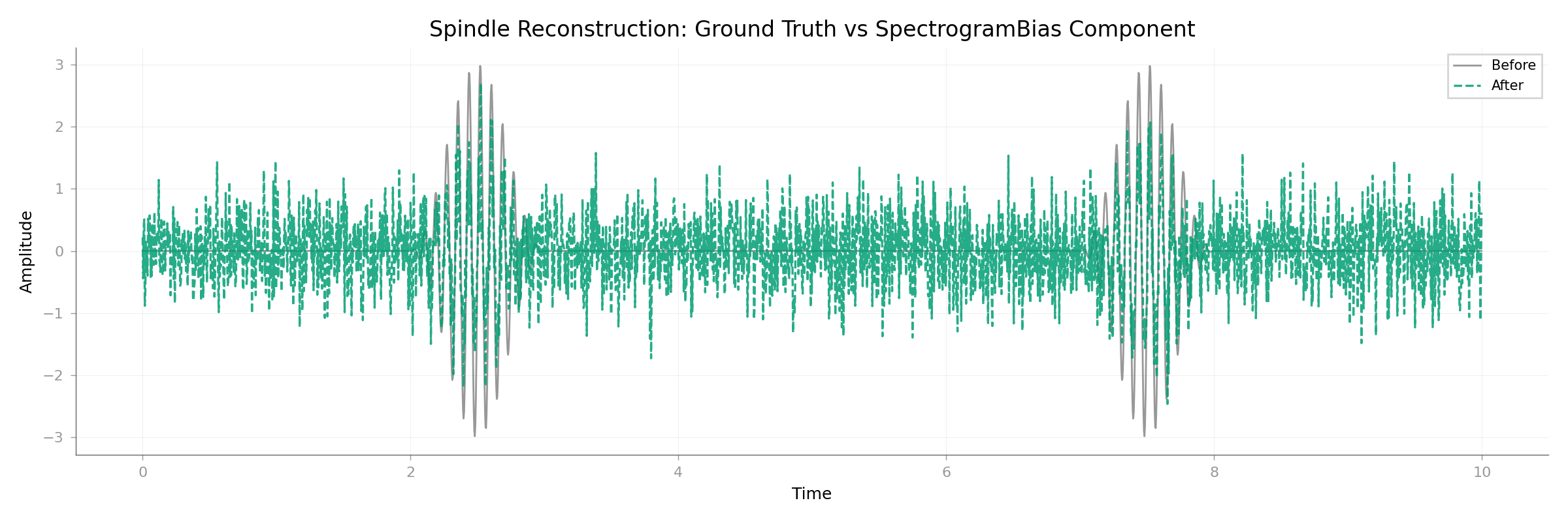
Correlation with ground truth: 0.512
Creating RawArray with float64 data, n_channels=1, n_times=2500
    Range : 0 ... 2499 =      0.000 ...     9.996 secs
Ready.
Creating RawArray with float64 data, n_channels=1, n_times=2500
    Range : 0 ... 2499 =      0.000 ...     9.996 secs
Ready.
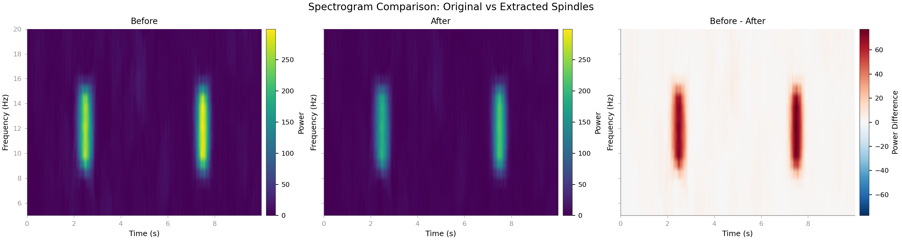
plot_spectrogram_comparison(
    raw_orig,
    raw_comp,
    picks=[0],
    times=raw_orig.times,
    fmin=5,
    fmax=20,
    show=False,
)
plt.gcf().suptitle("Spectrogram Comparison: Original vs Extracted Spindles")
plt.show()

# Plot comparison
plot_signal_overlay(
    signal_spindle,
    comp0_tf,
    times=times,
    title="Spindle Reconstruction: Ground Truth vs SpectrogramBias Component",
    scale_after=True,
    show=False,
)
plt.show()
Part 2: SpectrogramDenoiser + IterativeDSS (Adaptive)#
Automatically find TF regions with high energy
print("\n--- Part 2: Adaptive TF Masking (SpectrogramDenoiser) ---")

# SpectrogramDenoiser keeps only top percentile of TF energy
spec_denoiser = SpectrogramDenoiser(
    threshold_percentile=90,  # Keep top 10%
    nperseg=128,
    noverlap=96,
)

# Use with IterativeDSS on original spindle data
idss_spec = IterativeDSS(denoiser=spec_denoiser, n_components=2, max_iter=3)

idss_spec.fit(raw_spindle)
print("IterativeDSS with SpectrogramDenoiser converged")

sources_idss = idss_spec.transform(raw_spindle)
comp0_idss = sources_idss[0]

if np.corrcoef(comp0_idss, signal_spindle)[0, 1] < 0:
    comp0_idss *= -1

corr_idss = np.corrcoef(comp0_idss, signal_spindle)[0, 1]
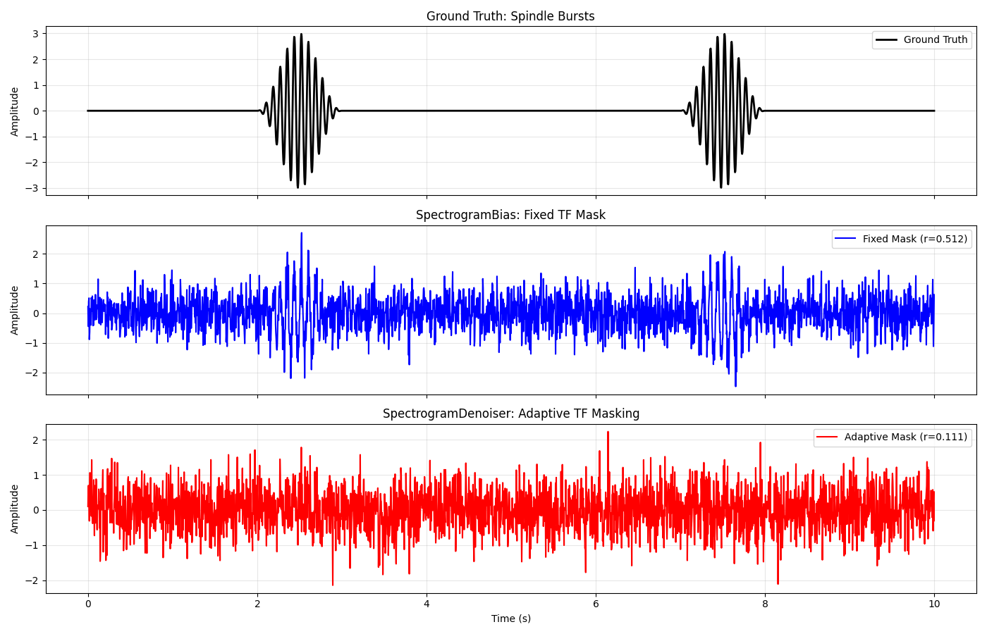
print(f"Correlation with ground truth: {corr_idss:.3f}")

# Compare both methods
fig, axes = plt.subplots(3, 1, figsize=(14, 9), sharex=True)

axes[0].plot(times, signal_spindle, "k", linewidth=2, label="Ground Truth")
axes[0].set_title("Ground Truth: Spindle Bursts")
axes[0].set_ylabel("Amplitude")
axes[0].legend()
axes[0].grid(True, alpha=0.3)

axes[1].plot(
    times,
    comp0_tf * (np.std(signal_spindle) / np.std(comp0_tf)),
    "b",
    label=f"Fixed Mask (r={corr_tf:.3f})",
)
axes[1].set_title("SpectrogramBias: Fixed TF Mask")
axes[1].set_ylabel("Amplitude")
axes[1].legend()
axes[1].grid(True, alpha=0.3)

axes[2].plot(
    times,
    comp0_idss * (np.std(signal_spindle) / np.std(comp0_idss)),
    "r",
    label=f"Adaptive Mask (r={corr_idss:.3f})",
)
axes[2].set_title("SpectrogramDenoiser: Adaptive TF Masking")
axes[2].set_xlabel("Time (s)")
axes[2].set_ylabel("Amplitude")
axes[2].legend()
axes[2].grid(True, alpha=0.3)

plt.tight_layout()
plt.show()
--- Part 2: Adaptive TF Masking (SpectrogramDenoiser) ---
IterativeDSS with SpectrogramDenoiser converged
Correlation with ground truth: 0.311
Part 3: Real MEG Gamma Bursts (Somato Dataset)#
Extract transient gamma oscillations
print("\n--- Part 3: Real MEG Data (Gamma Bursts) ---")

# Download somato dataset (will skip if already downloaded)
data_path = somato.data_path(verbose=True)
raw_path = data_path / "sub-01" / "meg" / "sub-01_task-somato_meg.fif"

raw_somato = mne.io.read_raw_fif(raw_path, preload=True, verbose=False)
raw_somato.pick_types(meg="grad", eeg=False, eog=False, stim=False, exclude="bads")
# Use broader band and keep more data
raw_somato.filter(1, 100, fir_design="firwin", verbose=False)  # Broad band first
raw_somato.crop(0, 60)  # 60 seconds for more data

print(f"MEG Data: {len(raw_somato.ch_names)} channels, {raw_somato.times[-1]:.1f}s")

# Apply SpectrogramDenoiser
spec_denoiser_meg = SpectrogramDenoiser(
    threshold_percentile=95,  # Top 5% of TF energy
    nperseg=256,
)

idss_meg = IterativeDSS(denoiser=spec_denoiser_meg, n_components=3, max_iter=3)

idss_meg.fit(raw_somato)
print("\nIterativeDSS on MEG data converged")

# Visualize (skip topomaps - use time series)
sources_meg = idss_meg.transform(raw_somato)

# Create Raw for visualization
comp_raw_meg = mne.io.RawArray(
    sources_meg[:1], mne.create_info(1, raw_somato.info["sfreq"], "misc")
)
raw_single_meg = raw_somato.copy().pick([0])

# --- Time Course Comparison ---
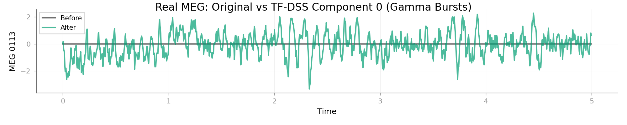
plot_channel_time_course_comparison(
    raw_single_meg,
    comp_raw_meg,
    picks=[0],
    times=raw_single_meg.times,
    start=0,
    stop=int(5 * raw_single_meg.info["sfreq"]),
    show=False,
)
plt.gcf().suptitle("Real MEG: Original vs TF-DSS Component 0 (Gamma Bursts)")
plt.show()

# --- Spectrogram Comparison (Pre/Post) ---
# Compares broadband raw data vs the broadband component
--- Part 3: Real MEG Data (Gamma Bursts) ---
NOTE: pick_types() is a legacy function. New code should use inst.pick(...).
MEG Data: 204 channels, 60.0s

IterativeDSS on MEG data converged
Creating RawArray with float64 data, n_channels=1, n_times=18019
    Range : 0 ... 18018 =      0.000 ...    59.999 secs
Ready.
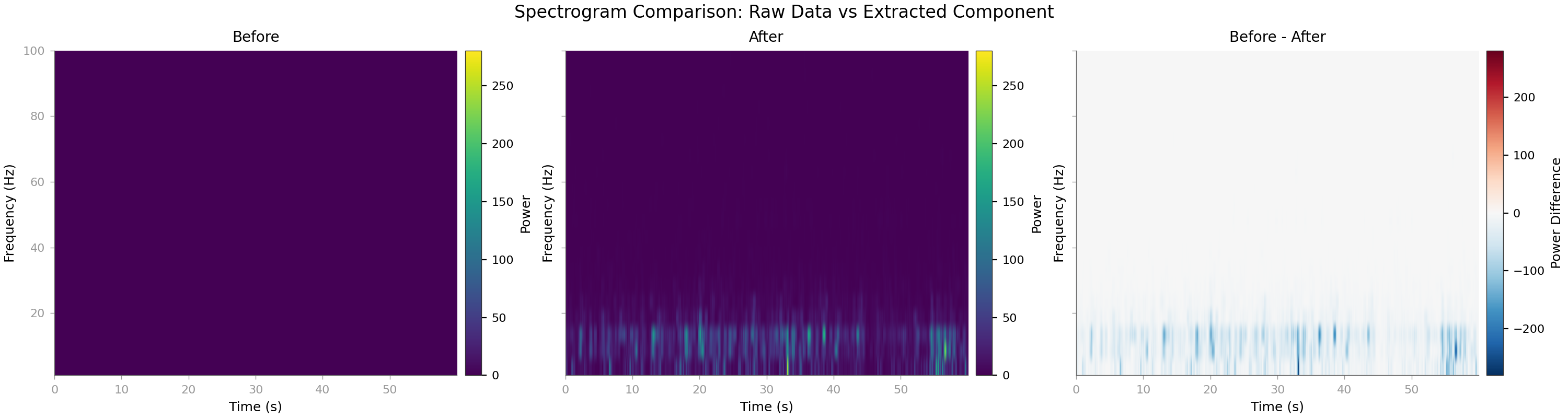
plot_spectrogram_comparison(
    raw_single_meg,
    comp_raw_meg,
    picks=[0],
    times=raw_single_meg.times,
    fmin=1,
    fmax=100,
    show=False,
)
plt.gcf().suptitle("Spectrogram Comparison: Raw Data vs Extracted Component")
plt.show()

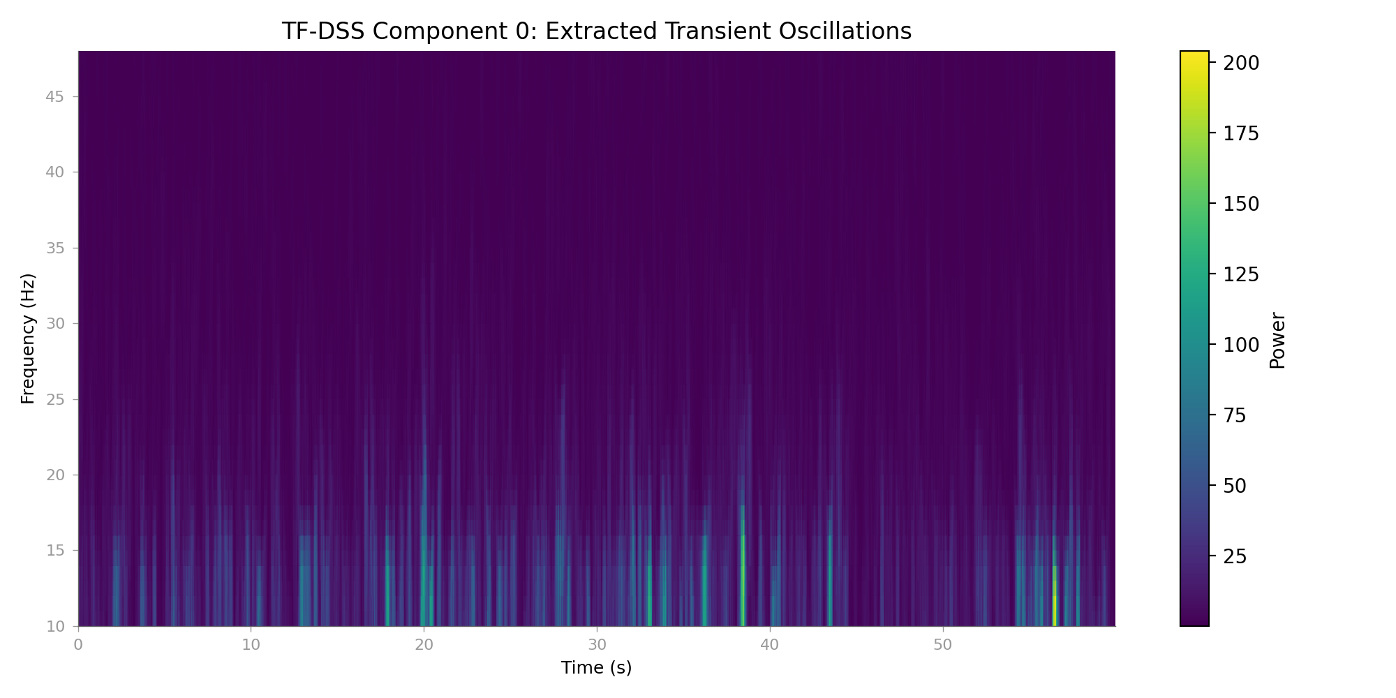
# --- Component Spectrogram (Single Component TFR) ---
# Zoom into the component's frequency content
freqs = np.arange(10, 50, 2)
plot_component_spectrogram(
    sources_meg[0],
    sfreq=raw_somato.info["sfreq"],
    freqs=freqs,
    title="TF-DSS Component 0: Extracted Transient Oscillations",
    show=False,
)
plt.show()

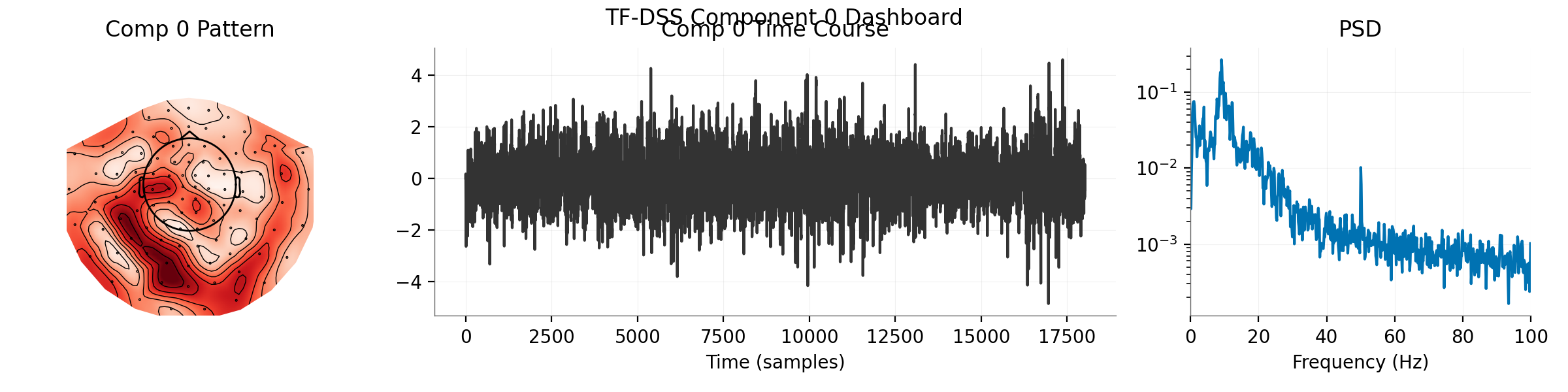
# --- Full Component Summary (with Topomaps!) ---
# Now that we have info, we can show topomaps
# Note: IterativeDSS stores patterns, so plot_component_summary can extract them.
print("\nPlotting full component dashboard (including Topomaps)...")
Plotting full component dashboard (including Topomaps)...
plot_component_summary(
    idss_meg,
    data=raw_somato,
    info=raw_somato.info,
    picks=np.arange(len(raw_somato.ch_names)),
    n_components=1,
    show=False,
)
plt.gcf().suptitle("TF-DSS Component 0 Dashboard")
plt.show()

print("\nSuccessfully extracted transient gamma oscillations using TF masking!")
Successfully extracted transient gamma oscillations using TF masking!
Total running time of the script: (0 minutes 11.700 seconds)