Efficiency Benchmark: DSS vs PCA, ICA, and Averaging.

This example demonstrates the superior efficiency of DSS in recovering evoked responses compared to standard methods.

It compares the best single channel, channel averaging, PCA, FastICA, and DSS. The metric is an SNR proxy defined as the variance of the trial-averaged signal. Because uncorrelated noise shrinks with averaging, higher variance in the average indicates better recovery of the phase-locked response.

Authors: Sina Esmaeili (sina.esmaeili@umontreal.ca)

Hamza Abdelhedi (hamza.abdelhedi@umontreal.ca)

import matplotlib.pyplot as plt
import mne
import numpy as np
from sklearn.decomposition import PCA, FastICA

from mne_denoise.dss import DSS, AverageBias

print(__doc__)

1. Generate Synthetic Evoked Response Data

We simulate a dataset with a known “Evoked” source (M100-like waveform) embedded in spatially correlated noise. The simulation uses 60 channels, 350 time points, and 100 epochs, with signal power set to 5.0 and noise power set to 3.0.

n_epochs = 100
n_channels = 60
n_times = 350
sfreq = 500
times = np.linspace(-0.2, 0.5, n_times)

# create M100-like waveform (Gabor patch)
evoked_src = np.exp(-((times - 0.1) ** 2) / (2 * 0.03**2)) * np.sin(
    2 * np.pi * 10 * times
)
evoked_src /= np.std(evoked_src)

# Spatial pattern (e.g., bilateral dipoles)
rng = np.random.default_rng(42)
pattern = np.sin(np.linspace(0, 2 * np.pi, n_channels))
pattern /= np.linalg.norm(pattern)

# Generate Data
data = np.zeros((n_epochs, n_channels, n_times))
signal_power = 5.0
noise_power = 3.0

print("Generating synthetic data...")
for i in range(n_epochs):
    # Fixed signal (Evoked)
    sig = signal_power * np.outer(pattern, evoked_src)

    # Random noise (uncorrelated across trials, but some spatial structure)
    # We mix random noise to create spatial correlation
    noise_raw = rng.standard_normal((n_channels + 10, n_times))
    mix_noise = rng.standard_normal((n_channels, n_channels + 10))
    noise = noise_power * (mix_noise @ noise_raw)
    noise /= np.std(noise)

    data[i] = sig + noise

# Create MNE Epochs for convenience
info = mne.create_info(n_channels, sfreq, "eeg")
epochs = mne.EpochsArray(data, info, tmin=-0.2, verbose=False)

# Compute true Evoked for reference
true_evoked_data = signal_power * evoked_src

print(f"Data shape: {epochs.get_data().shape} (Epochs, Channels, Times)")

Generating synthetic data...
Data shape: (100, 60, 350) (Epochs, Channels, Times)

Helper: Compute SNR Proxy

def compute_snr_proxy(data_3d):
    """
    Compute SNR proxy: Variance of the trial-averaged signal.

    Parameters
    ----------
    data_3d : ndarray (n_epochs, n_ch/n_comp, n_times)

    Returns
    -------
    snr : float (for best channel/component)
    best_idx : int
    avg_waveform : ndarray (n_times,)
    """
    # Average over epochs (Evoked response)
    evoked = data_3d.mean(axis=0)

    # Calculate variance (power) of the evoked response for each channel/component
    power = np.var(evoked, axis=1)

    best_idx = np.argmax(power)
    best_snr = power[best_idx]
    best_waveform = evoked[best_idx]

    return best_idx, best_snr, best_waveform

Method 1: Best Single Channel

print("\nRunning Method 1: Best Single Channel...")
best_ch_idx, snr_best_ch, wave_best_ch = compute_snr_proxy(epochs.get_data())
print(f"  Best Channel: #{best_ch_idx}, SNR: {snr_best_ch:.2f}")

Running Method 1: Best Single Channel...
  Best Channel: #44, SNR: 0.87

Method 2: Averaging Best 20 Channels

print("\nRunning Method 2: Average of Best 20 Channels...")
# Rank channels by evoked power
evoked_power = np.var(epochs.get_data().mean(axis=0), axis=1)
best_20_indices = np.argsort(evoked_power)[-20:]

# Extract data for these 20 channels
data_20 = epochs.get_data()[:, best_20_indices, :]

# Align signs to avoid cancellation!
# We align to the single best channel (which is one of them)
best_ch_idx_local = np.argmax(evoked_power[best_20_indices])
ref_wave = data_20[:, best_ch_idx_local, :].mean(axis=0)

aligned_data_20 = data_20.copy()
for i in range(20):
    # Check correlation with reference
    ch_wave = data_20[:, i, :].mean(axis=0)
    if np.corrcoef(ch_wave, ref_wave)[0, 1] < 0:
        aligned_data_20[:, i, :] *= -1

# Average spatially (across channels) -> (n_epochs, 1, n_times)
# effectively creating a "virtual channel"
data_avg_20 = aligned_data_20.mean(axis=1, keepdims=True)

_, snr_avg_20, wave_avg_20 = compute_snr_proxy(data_avg_20)
print(f"  Average 20 SNR: {snr_avg_20:.2f}")

Running Method 2: Average of Best 20 Channels...
  Average 20 SNR: 0.77

Method 3: PCA (sklearn)

print("\nRunning Method 3: PCA...")
# Reshape to (n_samples_total, n_channels) for sklearn
# PCA finds directions of maximum TOTAL variance (Signal + Noise)
X_concat = np.transpose(epochs.get_data(), (0, 2, 1)).reshape(
    -1, n_channels
)  # (n_epochs*n_times, n_ch)

pca = PCA(n_components=10, random_state=42)
X_pca = pca.fit_transform(X_concat)

# Reshape back to (n_epochs, n_times, n_comps) -> (n_epochs, n_comps, n_times)
data_pca = X_pca.reshape(n_epochs, n_times, 10).transpose(0, 2, 1)

best_pc_idx, snr_pca, wave_pca = compute_snr_proxy(data_pca)
print(f"  Best PC: #{best_pc_idx}, SNR: {snr_pca:.2f}")
# Fix sign if anti-correlated
if np.corrcoef(wave_pca, true_evoked_data)[0, 1] < 0:
    wave_pca *= -1

Running Method 3: PCA...
  Best PC: #0, SNR: 25.09

Method 4: FastICA (sklearn)

print("\nRunning Method 4: FastICA...")
# ICA tries to find independent components (non-Gaussian)
# Often effective for artifacts, effectively random for Gaussians
ica = FastICA(n_components=10, random_state=42)
X_ica = ica.fit_transform(X_concat)

data_ica = X_ica.reshape(n_epochs, n_times, 10).transpose(0, 2, 1)

best_ic_idx, snr_ica, wave_ica = compute_snr_proxy(data_ica)
print(f"  Best IC: #{best_ic_idx}, SNR: {snr_ica:.2f}")

# Re-scale ICA (since ICA has arbitrary scale) to match
# best channel magnitude for fair visual comparison
scaling = np.std(wave_best_ch) / np.std(wave_ica)
wave_ica *= scaling
if np.corrcoef(wave_ica, true_evoked_data)[0, 1] < 0:
    wave_ica *= -1

Running Method 4: FastICA...
  Best IC: #2, SNR: 0.96

Method 5: DSS (Trial Averaging)

print("\nRunning Method 5: DSS (Our Method)...")
# We use AverageBias (default axis='epochs'), which
# specifically optimizes for the evoked response
# (maximizing ratio of Mean / Variance).

dss = DSS(bias=AverageBias(), n_components=5)
dss.fit(epochs)
data_dss = dss.transform(epochs)  # returns (n_epochs, n_comps, n_times)

# Component 0 is guaranteed to be the best by DSS design (eigenvalue sorting)
best_dss_idx = 0
_, snr_dss, wave_dss = compute_snr_proxy(data_dss)
# But let's pick strictly by our proxy just in case
best_dss_idx, snr_dss, wave_dss = compute_snr_proxy(data_dss)
print(f"  Best DSS: #{best_dss_idx}, SNR: {snr_dss:.2f}")

# Re-scale DSS pattern if sign flipped (arbitrary sign)
if np.corrcoef(wave_dss, true_evoked_data)[0, 1] < 0:
    wave_dss *= -1

# Scale for visual comparison (DSS is scale-invariant/whitened)
wave_dss *= np.std(wave_best_ch) / np.std(wave_dss)

Running Method 5: DSS (Our Method)...
/home/runner/work/mne-denoise/mne-denoise/mne_denoise/dss/linear.py:496: RuntimeWarning: Epochs are not baseline corrected, covariance matrix may be inaccurate
  baseline_cov = mne.compute_covariance(inst, method=method, **kws)
/home/runner/work/mne-denoise/mne-denoise/mne_denoise/dss/linear.py:498: RuntimeWarning: Epochs are not baseline corrected, covariance matrix may be inaccurate
  biased_cov = mne.compute_covariance(biased_inst, method=method, **kws)
  Best DSS: #0, SNR: 0.96

3. Visualization: Bar Chart Comparison

methods = ["Best Channel", "Avg 20 Ch", "Best PCA", "Best ICA", "DSS"]
snrs = [
    snr_best_ch,
    snr_avg_20,
    snr_pca,
    snr_ica,
    snr_dss,
]  # Raw variance values might vary due to scale
# We normalize improvements relative to Best Channel = 1.0
relative_improvement = np.array(snrs) / snrs[0]


# IMPORTANT: ICA/PCA/DSS scales are arbitrary.
# Comparing "Raw Variance" (which is SNR Proxy *if* noise is
# constant) is tricky across methods
# if they apply different gains.
# However, "SNR" in the context of Evoked BCI is usually
# (Power of Avg) / (Residual Variance).
# Our proxy `var(mean)` assumes noise cancels out exactly or similarly.
# A more robust SNR is (Power of Signal) / (Power of Noise).
#
# Let's compute a "Real SNR" metric for the plot:
# SNR = Var(Evoked) / Var(Residual)
def compute_true_snr(data_3d, idx):
    evoked = data_3d.mean(axis=0)[idx]
    residual = data_3d[:, idx, :] - evoked[None, :]
    return np.var(evoked) / np.var(residual)


print("\nCalculating True SNR (Signal / Residual)...")
true_snr_vals = []
true_snr_vals.append(compute_true_snr(epochs.get_data(), best_ch_idx))
true_snr_vals.append(compute_true_snr(data_avg_20, 0))
true_snr_vals.append(compute_true_snr(data_pca, best_pc_idx))
true_snr_vals.append(compute_true_snr(data_ica, best_ic_idx))
true_snr_vals.append(compute_true_snr(data_dss, best_dss_idx))

relative_improvement_true = np.array(true_snr_vals) / true_snr_vals[0]

fig, ax = plt.subplots(figsize=(10, 6))
bars = ax.bar(
    methods,
    relative_improvement_true,
    color=["gray", "gray", "orange", "purple", "blue"],
    alpha=0.8,
    edgecolor="k",
)

# Highlight DSS
bars[-1].set_alpha(1.0)
bars[-1].set_linewidth(2)

# Add labels
for bar, val in zip(bars, relative_improvement_true):
    height = bar.get_height()
    ax.text(
        bar.get_x() + bar.get_width() / 2.0,
        height + 0.1,
        f"{val:.1f}x",
        ha="center",
        va="bottom",
        fontweight="bold",
        fontsize=12,
    )

ax.axhline(1.0, color="r", linestyle="--", alpha=0.5, label="Baseline")
ax.set_ylabel("SNR Improvement (Relative to Best Channel)")
ax.set_title("Denoising Efficiency Comparison (Higher is Better)")
ax.legend()
plt.tight_layout()
plt.show()

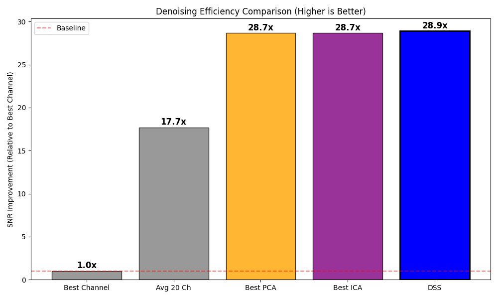
Calculating True SNR (Signal / Residual)...

4. Visualization: Time Course Comparison

Overlay the recovered waveforms.

fig, ax = plt.subplots(figsize=(12, 6))

t = times
ax.plot(
    t,
    wave_best_ch / np.max(np.abs(wave_best_ch)),
    "k--",
    alpha=0.4,
    label="Best Single Channel",
)
ax.plot(
    t,
    wave_avg_20 / np.max(np.abs(wave_avg_20)),
    "g-.",
    alpha=0.6,
    label="Avg 20 Channels",
)
ax.plot(
    t, wave_pca / np.max(np.abs(wave_pca)), color="orange", alpha=0.6, label="Best PCA"
)
# ax.plot(t, wave_ica, color='purple', alpha=0.6,
#         label='Best ICA')  # ICA often poor for this
ax.plot(
    t, wave_dss / np.max(np.abs(wave_dss)), "b", linewidth=2.5, label="DSS (Optimal)"
)

# Plot ground truth
ax.plot(
    t,
    evoked_src / np.max(np.abs(evoked_src)),
    "r:",
    linewidth=2,
    alpha=0.8,
    label="True Source",
)

ax.set_xlabel("Time (s)")
ax.set_ylabel("Normalized Amplitude")
ax.set_title("Recovered Evoked Responses")
ax.legend(loc="upper right")
ax.grid(True, linestyle=":")

plt.tight_layout()
plt.show()

print("\nExample 10 Complete! DSS should show the highest SNR improvement.")

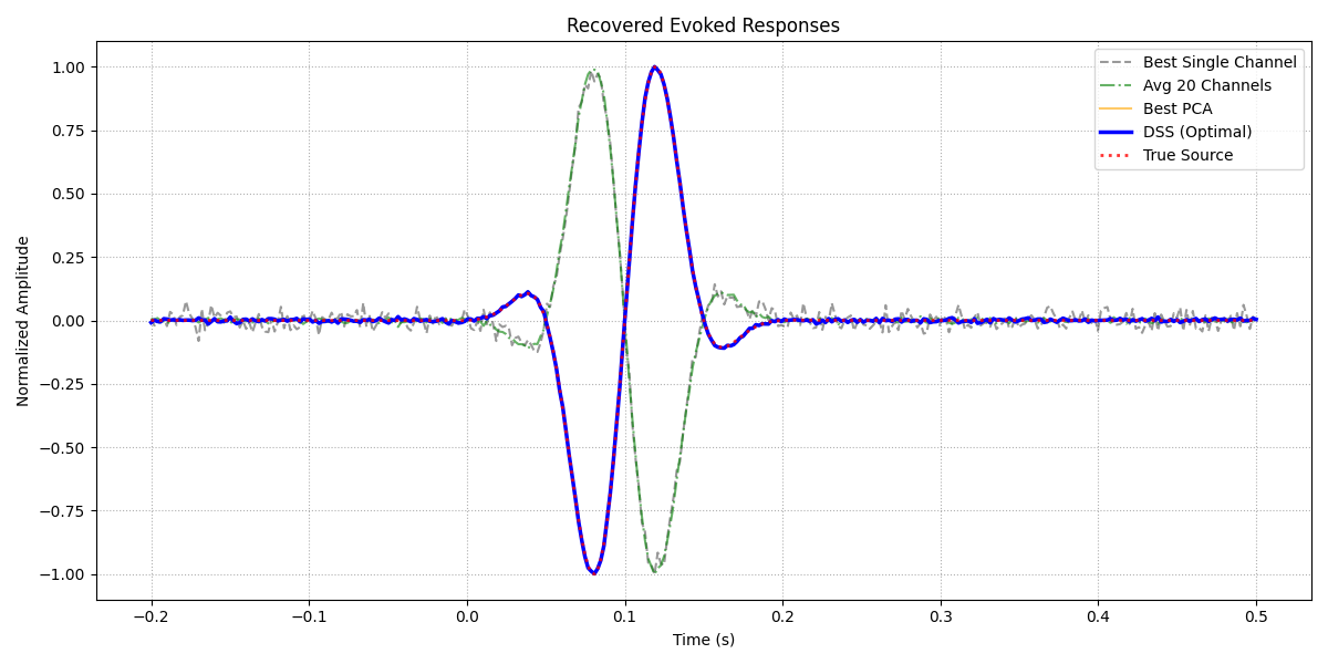
Example 10 Complete! DSS should show the highest SNR improvement.