ZapLine: Parameter Tuning and Real Data.

This example shows how the main ZapLine tuning parameters change the cleaning behavior on synthetic data, then applies the same workflow to a real NoiseTools MEG recording.

Authors: Sina Esmaeili (sina.esmaeili@umontreal.ca)

Hamza Abdelhedi (hamza.abdelhedi@umontreal.ca)

Imports

from pathlib import Path
from urllib.request import urlretrieve

import matplotlib.pyplot as plt
import mne
import numpy as np
from scipy import signal
from scipy.io import loadmat

from mne_denoise.viz import (
    plot_component_cleaning_summary,
    plot_component_patterns,
    plot_component_score_curve,
    plot_psd_comparison,
)
from mne_denoise.zapline import ZapLine

NOISETOOLS_BASE_URL = "http://audition.ens.fr/adc/NoiseTools/DATA"


def _find_repo_root():
    """Return the repository root for this example."""
    starts = []
    if "__file__" in globals():
        starts.append(Path(__file__).resolve())
    starts.append(Path.cwd().resolve())

    for start in starts:
        current = start if start.is_dir() else start.parent
        for candidate in (current, *current.parents):
            mne_ok = (candidate / "mne_denoise").exists()
            ex_ok = (candidate / "examples").exists()
            if mne_ok and ex_ok:
                return candidate

    raise FileNotFoundError("Could not locate the repository root.")


def _load_or_fetch_data_file(name):
    """Return one ZapLine example data file, downloading it if needed."""
    path = _find_repo_root() / "examples" / "zapline" / "data" / name
    if path.exists():
        return path

    path.parent.mkdir(parents=True, exist_ok=True)
    url = f"{NOISETOOLS_BASE_URL}/{name}"
    print(f"Downloading {name} to {path}...")
    urlretrieve(url, str(path))
    return path

Part 1: n_remove Parameter

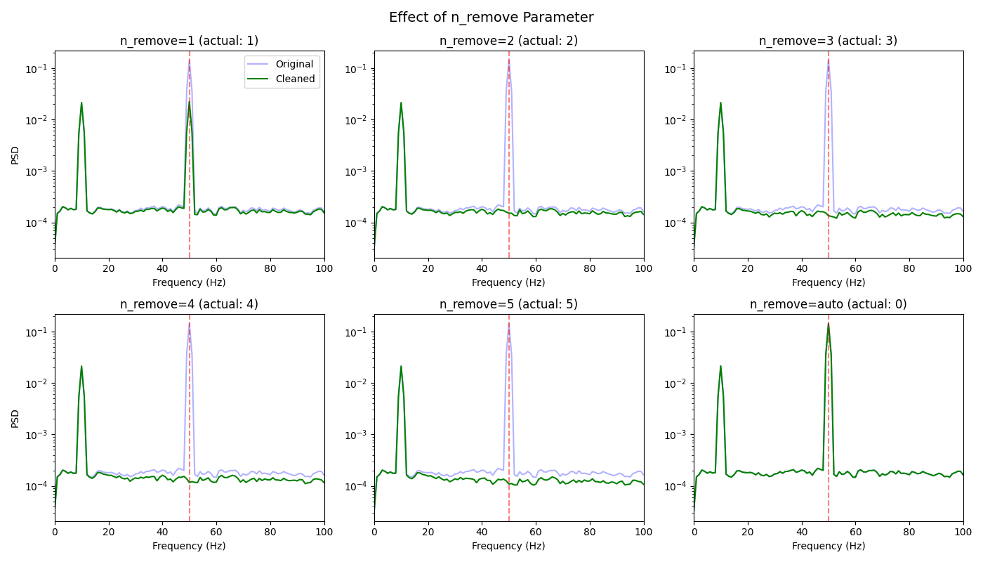
The n_remove parameter controls how many spatial components are removed. Too few: line noise remains. Too many: neural signal lost.

print("Part 1: Exploring n_remove parameter")

# Generate synthetic data with multiple line noise sources
sfreq = 1000
duration = 5
n_channels = 16
n_times = int(sfreq * duration)
t = np.arange(n_times) / sfreq

rng = np.random.RandomState(42)

# Create 3 distinct line noise sources (simulating multiple power sources)
n_line_sources = 3
line_patterns = rng.randn(n_channels, n_line_sources)
for i in range(n_line_sources):
    line_patterns[:, i] /= np.linalg.norm(line_patterns[:, i])

# Neural pattern
neural_pattern = rng.randn(n_channels)
neural_pattern /= np.linalg.norm(neural_pattern)

# Generate data
neural_source = np.sin(2 * np.pi * 10 * t)
line_sources = np.zeros((n_line_sources, n_times))
for i in range(n_line_sources):
    phase = rng.uniform(0, 2 * np.pi)
    amp = 2.0 - i * 0.5  # Decreasing amplitude
    line_sources[i] = amp * np.sin(2 * np.pi * 50 * t + phase)

data = np.zeros((n_channels, n_times))
for i in range(n_channels):
    data[i] = neural_pattern[i] * neural_source
    for j in range(n_line_sources):
        data[i] += line_patterns[i, j] * line_sources[j]
    data[i] += rng.randn(n_times) * 0.3

print(f"Data with {n_line_sources} line noise sources")

Part 1: Exploring n_remove parameter
Data with 3 line noise sources

Compare Different n_remove Values

Small values tend to leave narrowband noise behind. Larger values clean more aggressively, but eventually start removing structure that is no longer just line noise.

fig, axes = plt.subplots(2, 3, figsize=(14, 8))

n_remove_values = [1, 2, 3, 4, 5, "auto"]

for idx, n_remove in enumerate(n_remove_values):
    row, col = idx // 3, idx % 3
    ax = axes[row, col]

    est = ZapLine(line_freq=50, sfreq=sfreq, n_remove=n_remove)
    est.fit(data)
    cleaned = est.transform(data)

    freqs, psd_orig = signal.welch(data, sfreq, nperseg=sfreq)
    freqs, psd_clean = signal.welch(cleaned, sfreq, nperseg=sfreq)

    ax.semilogy(freqs, np.mean(psd_orig, axis=0), "b-", alpha=0.3, label="Original")
    ax.semilogy(freqs, np.mean(psd_clean, axis=0), "g-", label="Cleaned")
    ax.axvline(50, color="r", linestyle="--", alpha=0.5)
    ax.set_xlim(0, 100)
    ax.set_title(f"n_remove={n_remove} (actual: {est.n_removed_})")
    ax.set_xlabel("Frequency (Hz)")

    if col == 0:
        ax.set_ylabel("PSD")
    if idx == 0:
        ax.legend()

plt.suptitle("Effect of n_remove Parameter", fontsize=14)
plt.tight_layout()
plt.show()

Part 2: nkeep Parameter (High Channel Count)

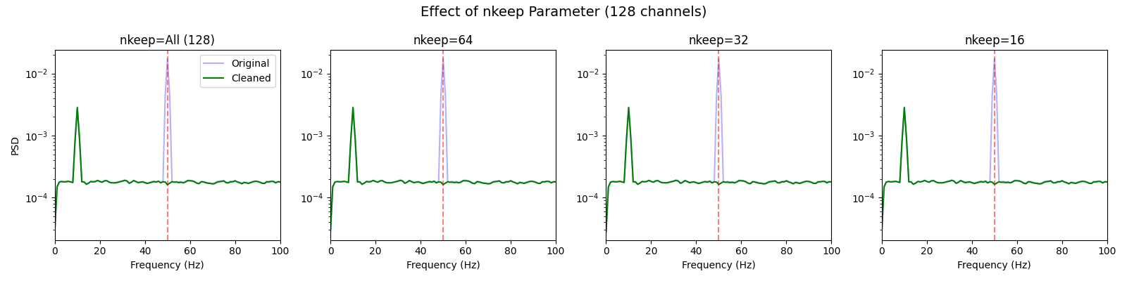
For data with many channels, the optional nkeep parameter reduces dimensionality before DSS to avoid overfitting.

print("\nPart 2: nkeep parameter for high-channel data")

# Create high-channel-count data
n_channels_high = 128
data_high = np.zeros((n_channels_high, n_times))

# Multiple line sources with different spatial patterns
n_line_sources = 2
line_patterns_high = rng.randn(n_channels_high, n_line_sources)
for i in range(n_line_sources):
    line_patterns_high[:, i] /= np.linalg.norm(line_patterns_high[:, i])

neural_pattern_high = rng.randn(n_channels_high)
neural_pattern_high /= np.linalg.norm(neural_pattern_high)

for i in range(n_channels_high):
    data_high[i] = neural_pattern_high[i] * neural_source
    for j in range(n_line_sources):
        data_high[i] += line_patterns_high[i, j] * line_sources[j]
    data_high[i] += rng.randn(n_times) * 0.3

print(f"High-channel data: {data_high.shape}")

Part 2: nkeep parameter for high-channel data
High-channel data: (128, 5000)

Compare Different nkeep Values

The nkeep parameter matters most when the channel count is high. It trades some spatial richness for a more stable low-rank DSS problem.

fig, axes = plt.subplots(1, 4, figsize=(16, 4))

nkeep_values = [None, 64, 32, 16]

for idx, nkeep in enumerate(nkeep_values):
    ax = axes[idx]

    est_high = ZapLine(line_freq=50, sfreq=sfreq, n_remove=2, nkeep=nkeep)
    est_high.fit(data_high)
    cleaned_high = est_high.transform(data_high)

    freqs, psd_orig = signal.welch(data_high, sfreq, nperseg=sfreq)
    freqs, psd_clean = signal.welch(cleaned_high, sfreq, nperseg=sfreq)

    ax.semilogy(freqs, np.mean(psd_orig, axis=0), "b-", alpha=0.3, label="Original")
    ax.semilogy(freqs, np.mean(psd_clean, axis=0), "g-", label="Cleaned")
    ax.axvline(50, color="r", linestyle="--", alpha=0.5)
    ax.set_xlim(0, 100)
    ax.set_title(f"nkeep={nkeep if nkeep else 'All (128)'}")
    ax.set_xlabel("Frequency (Hz)")

    if idx == 0:
        ax.set_ylabel("PSD")
        ax.legend()

plt.suptitle("Effect of nkeep Parameter (128 channels)", fontsize=14)
plt.tight_layout()
plt.show()

Part 3: Component Scores

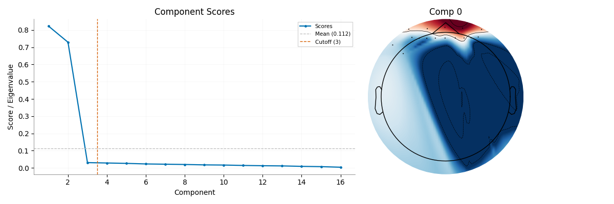
The eigenvalues (scores) indicate how much each component carries line noise. High scores = strong line noise. The selected components should be the ones that combine a strong narrowband signature with a plausible spatial pattern.

print("\nPart 3: Understanding component scores")

# Use a fixed removal count to guarantee selected components for pattern plots.
est_scores = ZapLine(line_freq=50, sfreq=sfreq, n_remove=3)
est_scores.fit(data)
plot_montage = mne.channels.make_standard_montage("standard_1020")
plot_info = mne.create_info(plot_montage.ch_names[:n_channels], sfreq, "eeg")
plot_info.set_montage(plot_montage)
plot_picks = np.arange(len(plot_info.ch_names))

# Use the reusable viz functions
fig, axes = plt.subplots(1, 2, figsize=(12, 4))
plot_component_score_curve(est_scores, ax=axes[0], show=False)
plot_component_patterns(
    est_scores,
    info=plot_info,
    picks=plot_picks,
    n_components=1,
    ax=axes[1],
    show=False,
)
plt.tight_layout()
plt.show()

Part 3: Understanding component scores

Part 4: Real MEG Data (NoiseTools)

Apply ZapLine to real MEG data from NoiseTools dataset. The file is cached under examples/zapline/data after the first run.

print("\nPart 4: Real MEG Data")

# Load data1.mat (MEG with large near-DC fluctuations)
data1_path = _load_or_fetch_data_file("data1.mat")
mat = loadmat(str(data1_path))
meg_data = mat["data"].T  # Transpose to (channels, times)
sfreq_meg = float(mat["sr"].flatten()[0])

# Demean
meg_data = meg_data - np.mean(meg_data, axis=1, keepdims=True)

print(f"Loaded data1.mat: {meg_data.shape}, sfreq={sfreq_meg} Hz")
print("MEG data with large near-DC fluctuations")

Part 4: Real MEG Data
Downloading data1.mat to /home/runner/work/mne-denoise/mne-denoise/examples/zapline/data/data1.mat...
Loaded data1.mat: (208, 40000), sfreq=1000.0 Hz
MEG data with large near-DC fluctuations

Apply ZapLine to MEG Data

# Apply ZapLine (60 Hz for this dataset)
est_meg = ZapLine(
    line_freq=60,
    sfreq=sfreq_meg,
    n_remove=2,  # As in MATLAB example
)
est_meg.fit(meg_data)
cleaned_meg = est_meg.transform(meg_data)

print(f"Components removed: {est_meg.n_removed_}")

Components removed: 2

Compare Before/After for MEG

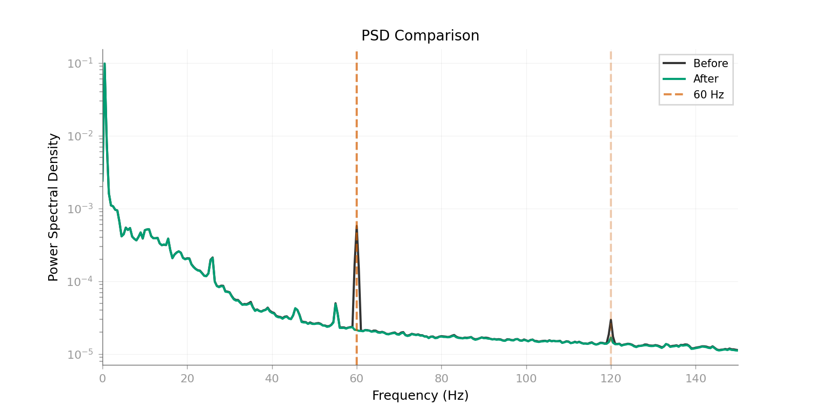
On the real recording, the relevant check is whether the 60 Hz peak drops sharply without flattening the rest of the broadband spectrum.

# Use reusable viz function for PSD comparison
plot_psd_comparison(
    meg_data,
    cleaned_meg,
    sfreq=sfreq_meg,
    line_freq=60,
    fmax=150,
    show=True,
)

<Figure size 1600x800 with 1 Axes>

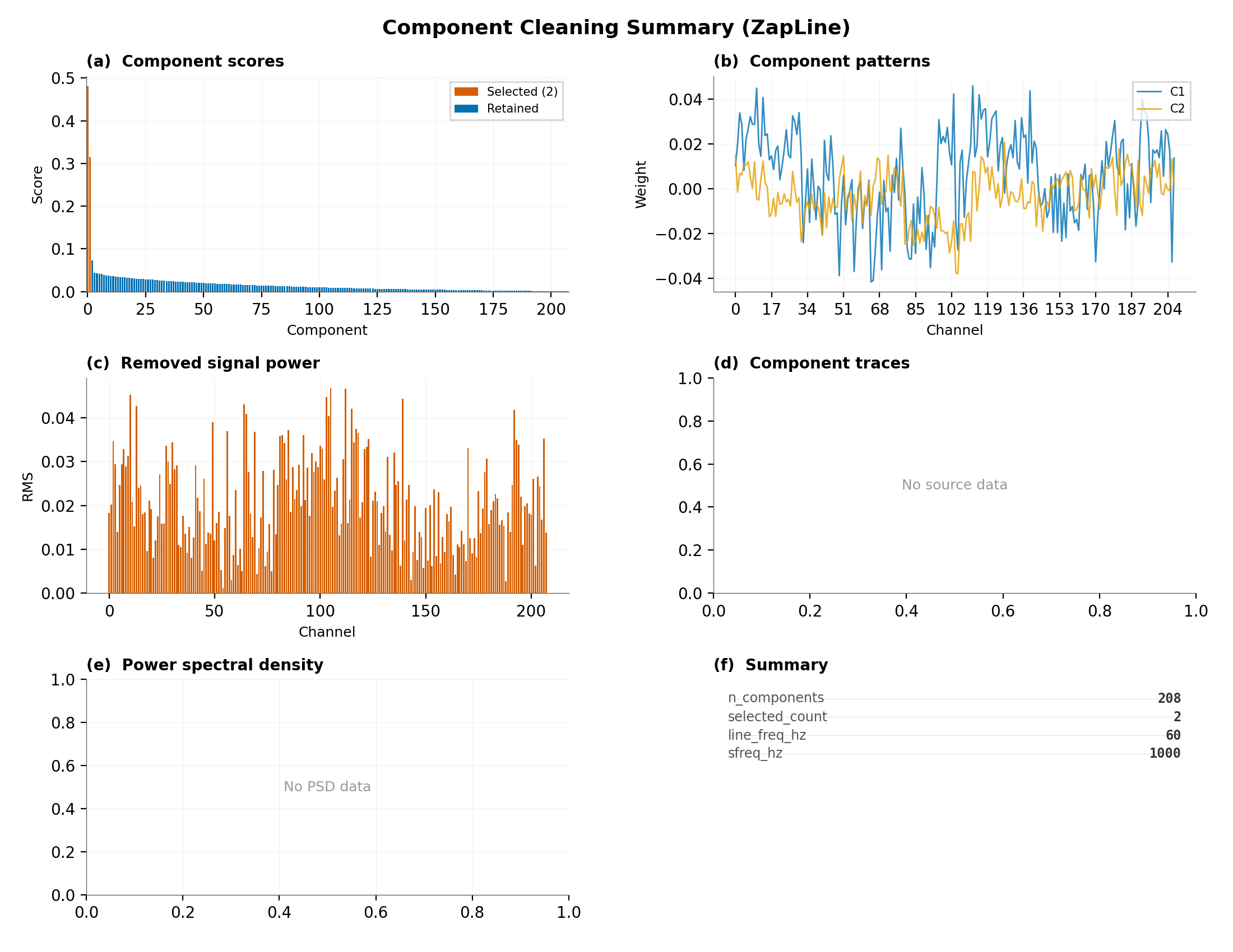
Component Cleaning Summary

plot_component_cleaning_summary(
    scores=getattr(est_meg, "scores_", getattr(est_meg, "eigenvalues_", None)),
    selected_count=getattr(est_meg, "n_removed_", 0),
    patterns=getattr(est_meg, "patterns_", None),
    removed=meg_data - cleaned_meg,
    sources=getattr(est_meg, "sources_", None),
    sfreq=sfreq_meg,
    line_freq=60,
    title="Component Cleaning Summary (ZapLine)",
    show=True,
)

/home/runner/work/mne-denoise/mne-denoise/mne_denoise/viz/theme.py:379: UserWarning: This figure includes Axes that are not compatible with tight_layout, so results might be incorrect.
  fig.tight_layout()

<Figure size 2200x1700 with 6 Axes>

Measure Reduction

freqs_meg, psd_orig_meg = signal.welch(meg_data, sfreq_meg, nperseg=int(sfreq_meg * 2))
_, psd_clean_meg = signal.welch(cleaned_meg, sfreq_meg, nperseg=int(sfreq_meg * 2))
idx_60 = np.argmin(np.abs(freqs_meg - 60))
power_60_orig = np.mean(psd_orig_meg[:, idx_60])
power_60_clean = np.mean(psd_clean_meg[:, idx_60])
reduction_db = 10 * np.log10(power_60_orig / power_60_clean)

print("\n=== MEG Results ===")
print(f"60 Hz power reduction: {reduction_db:.1f} dB")
print(f"Components removed: {est_meg.n_removed_}")

=== MEG Results ===
60 Hz power reduction: 14.3 dB
Components removed: 2

Conclusion

A practical starting point is to use n_remove="auto" or a small manual value such as 1 to 3, then increase it only if clear line-noise structure remains. nkeep becomes useful for high-channel recordings, threshold controls how aggressive automatic removal is, and n_harmonics matters most when the sampling rate is high enough for several harmonics to be present.