Joint DSS (Multi-Dataset Repeatability).

This example demonstrates Joint Denoising Source Separation (JDSS), a method for extracting components that are reproducible across multiple datasets.

JDSS is useful for finding sources that are consistent across subjects, consistent across recording blocks, or reproducible across repeated stimulus presentations.

The objective function is:

\[\max_w \frac{w^T R_{signal} w}{w^T R_{total} w}\]

where \(R_{signal} = Cov(\bar{X})\) is the covariance of the grand average and \(R_{total} = \frac{1}{N} \sum Cov(X_i)\) is the mean of the individual covariances.

Components with high eigenvalue are highly reproducible.

Reference:

de Cheveigné, A., & Parra, L. C. (2014). Joint decorrelation, a versatile tool for multichannel data analysis. NeuroImage, 98, 487-505.

Authors: Sina Esmaeili (sina.esmaeili@umontreal.ca)

Hamza Abdelhedi (hamza.abdelhedi@umontreal.ca)

Imports

import matplotlib.pyplot as plt
import numpy as np
from scipy import signal as sig

from mne_denoise.dss import DSS
from mne_denoise.dss.denoisers import AverageBias

Simulate Multi-Subject Data

We simulate five subjects that share one weak 10 Hz source while each subject also has strong pink noise with its own spatial pattern and additional low-amplitude sensor noise. This is exactly the regime where single-subject PCA or ICA struggles but JDSS can exploit cross-subject consistency.

print("=== Joint DSS Example ===\n")
print("Simulating 5 subjects with a shared 10 Hz source buried in noise...")

n_subjects = 5
n_channels = 16
n_times = 1000
sfreq = 250
times = np.arange(n_times) / sfreq

rng = np.random.RandomState(42)

# Common source: 10 Hz sine (signal)
common_source = np.sin(2 * np.pi * 10 * times)
common_source /= np.std(common_source)

# Common (but slightly varying) topography
base_topo = np.ones(n_channels)
base_topo[:8] = 1.5  # Stronger in first half of channels
base_topo /= np.linalg.norm(base_topo)

datasets = []
for subj in range(n_subjects):
    # Slightly perturb topography per subject (realistic)
    topo = base_topo + 0.1 * rng.randn(n_channels)
    topo /= np.linalg.norm(topo)

    # Signal component
    signal_part = np.outer(topo, common_source) * 1.0  # SNR ~ 1

    # Subject-specific noise (pink, strong)
    noise_topo = rng.randn(n_channels)
    noise_topo /= np.linalg.norm(noise_topo)
    noise_source = rng.randn(n_times)
    # Pink filter
    b, a = sig.butter(3, 0.1)
    noise_source = sig.filtfilt(b, a, noise_source)
    noise_source /= np.std(noise_source)
    noise_part = np.outer(noise_topo, noise_source) * 3.0  # 3x signal

    # Sensor noise
    sensor_noise = 0.3 * rng.randn(n_channels, n_times)

    data = signal_part + noise_part + sensor_noise
    datasets.append(data)

datasets = np.array(datasets)  # (n_subjects, n_channels, n_times)
print(f"Created {n_subjects} datasets of shape {datasets[0].shape}")
print("Signal amplitude: 1.0, Noise amplitude: 3.0 (SNR ~ 0.33)")

=== Joint DSS Example ===

Simulating 5 subjects with a shared 10 Hz source buried in noise...
Created 5 datasets of shape (16, 1000)
Signal amplitude: 1.0, Noise amplitude: 3.0 (SNR ~ 0.33)

Apply Joint DSS

JDSS finds the spatial filter that maximizes the ratio of “grand average variance” to “mean of individual variances”.

Note: DSS expects input shape (n_channels, n_times, n_epochs). We treat the 5 subjects as “epochs” for the purpose of finding reproducible components across subjects. So we transpose datasets from (n_subjects, n_ch, n_times) to (n_ch, n_times, n_subjects).

print("\nApplying JDSS (via DSS with group averaging)...")
datasets_dss = np.transpose(datasets, (1, 2, 0))  # (16, 1000, 5)

# Use 'epochs' axis to average over the 3rd dimension (which represents subjects here)
jdss = DSS(bias=AverageBias(axis="epochs"), n_components=3)
jdss.fit(datasets_dss)

print(f"Eigenvalues (repeatability scores): {jdss.eigenvalues_}")
print("  -> Score near 1.0 = highly reproducible.")
print("  -> Score near 0.0 = random noise.\n")

Applying JDSS (via DSS with group averaging)...
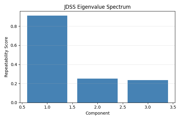
Eigenvalues (repeatability scores): [0.91191608 0.25192183 0.2334974 ]
  -> Score near 1.0 = highly reproducible.
  -> Score near 0.0 = random noise.

Extract Sources

Apply the learned filters to the data. Transform returns (n_components, n_times, n_subjects) because input was (n_ch, n_times, n_subjects)

sources = jdss.transform(datasets_dss)  # (3, 1000, 5)
sources = np.transpose(sources, (2, 0, 1))  # (n_subjects, n_components, n_times)

# Grand average of sources
ga_sources = np.mean(sources, axis=0)  # (n_components, n_times)

# Grand average of raw data (best channel)
ga_raw = np.mean(datasets, axis=0)
best_ch = np.argmax(np.var(ga_raw, axis=1))

Visualize Results

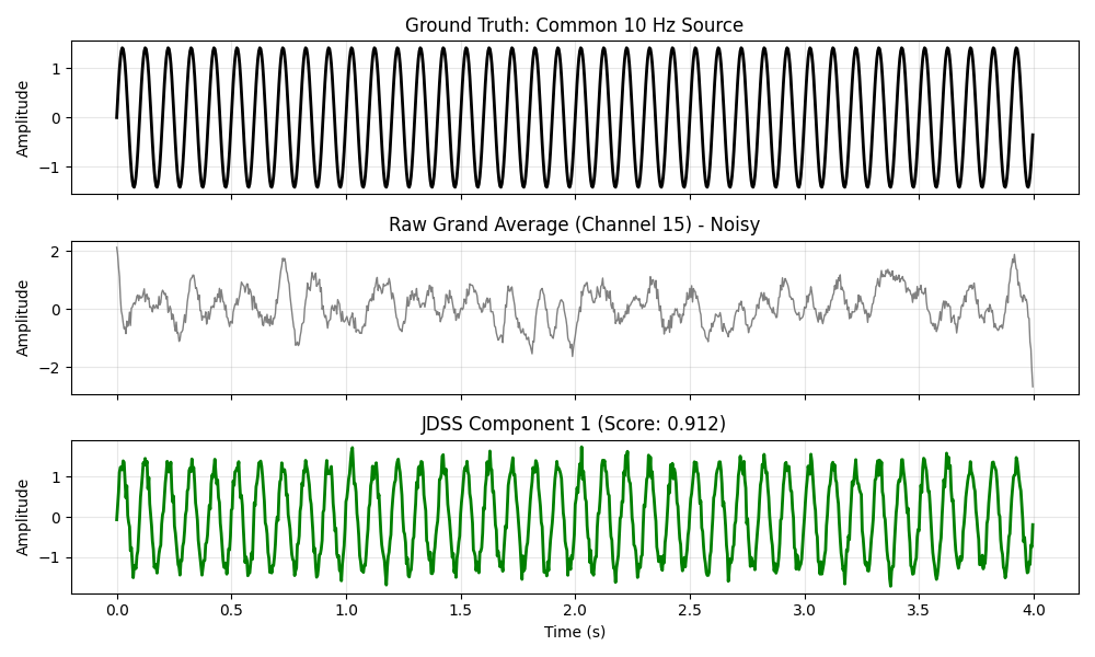
Compare the ground truth, raw grand average, and JDSS component 1.

fig, axes = plt.subplots(3, 1, figsize=(10, 6), sharex=True)

# Ground truth
axes[0].plot(times, common_source, "k", lw=2)
axes[0].set_ylabel("Amplitude")
axes[0].set_title("Ground Truth: Common 10 Hz Source")
axes[0].grid(True, alpha=0.3)

# Raw grand average (best channel)
axes[1].plot(times, ga_raw[best_ch], "gray", lw=1)
axes[1].set_ylabel("Amplitude")
axes[1].set_title(f"Raw Grand Average (Channel {best_ch}) - Noisy")
axes[1].grid(True, alpha=0.3)

# JDSS Component 1
# Flip sign if anti-correlated with ground truth
corr = np.corrcoef(ga_sources[0], common_source)[0, 1]
sign = np.sign(corr)
axes[2].plot(times, sign * ga_sources[0], "g", lw=2)
axes[2].set_ylabel("Amplitude")
axes[2].set_xlabel("Time (s)")
axes[2].set_title(f"JDSS Component 1 (Score: {jdss.eigenvalues_[0]:.3f})")
axes[2].grid(True, alpha=0.3)

plt.tight_layout()
plt.show()

Quantitative Evaluation

Compute correlation between JDSS output and ground truth.

corr_raw = np.abs(np.corrcoef(ga_raw[best_ch], common_source)[0, 1])
corr_jdss = np.abs(np.corrcoef(ga_sources[0], common_source)[0, 1])

print("=== Correlation with Ground Truth ===")
print(f"  Raw Grand Average (best channel): {corr_raw:.3f}")
print(f"  JDSS Component 1:                 {corr_jdss:.3f}")
print(f"\nJDSS improves recovery by {(corr_jdss - corr_raw) / corr_raw * 100:.1f}%")

=== Correlation with Ground Truth ===
  Raw Grand Average (best channel): 0.268
  JDSS Component 1:                 0.988

JDSS improves recovery by 268.5%

Per-Subject Sources

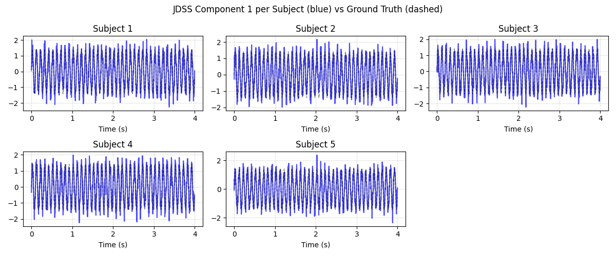
Show that JDSS sources are consistent across subjects.

fig, axes = plt.subplots(2, 3, figsize=(12, 5))
for i, ax in enumerate(axes.flat):
    if i < n_subjects:
        src = sources[i, 0]
        # Align sign
        if np.corrcoef(src, common_source)[0, 1] < 0:
            src = -src
        ax.plot(times, src, "b", alpha=0.7)
        ax.plot(times, common_source, "k--", alpha=0.5, lw=1)
        ax.set_title(f"Subject {i + 1}")
        ax.set_xlabel("Time (s)")
        ax.grid(True, alpha=0.3)
    else:
        ax.axis("off")

fig.suptitle("JDSS Component 1 per Subject (blue) vs Ground Truth (dashed)")
plt.tight_layout()
plt.show()

Eigenvalue Spectrum

The first eigenvalue should be much larger than the rest.

plt.figure(figsize=(6, 4))
plt.bar(range(1, len(jdss.eigenvalues_) + 1), jdss.eigenvalues_, color="steelblue")
plt.xlabel("Component")
plt.ylabel("Repeatability Score")
plt.title("JDSS Eigenvalue Spectrum")
plt.grid(True, alpha=0.3, axis="y")
plt.tight_layout()
plt.show()

Conclusion

JDSS successfully extracted the common 10 Hz signal even though the signal was weaker than the noise, the noise patterns varied across subjects, and the signal topographies were only approximately aligned. That is exactly the setting where a shared group-level component model is useful.