Fundamentals of DSS.#

This tutorial introduces Denoising Source Separation (DSS), a technique for extracting brain sources based on a specific criterion of “interestingness” (bias).

Unlike PCA, which finds components of high variance, or ICA, which finds components of high non-Gaussianity, DSS finds components that maximize a user-defined Bias.

The core optimization is:

\[\max_w \frac{w^T R_{biased} w}{w^T R_{baseline} w}\]

where \(R_{biased}\) is the covariance of the signal of interest and \(R_{baseline}\) is the covariance of the raw data or noise.

This allows DSS to be extremely flexible. The “Bias” defines what you are looking for. Typical biases include trial averaging for stimulus-evoked responses, bandpass filtering for oscillatory sources, and time masking for artifact removal.

This tutorial demonstrates the “Hello World” of DSS: extracting a repetitive signal buried in noise using the Trial Average Bias.

Authors: Sina Esmaeili (sina.esmaeili@umontreal.ca)

Hamza Abdelhedi (hamza.abdelhedi@umontreal.ca)

Imports#

import contextlib
import os

import mne
import numpy as np
from mne.datasets import sample

from mne_denoise.dss import DSS, AverageBias, BandpassBias
from mne_denoise.viz import (
    plot_component_patterns,
    plot_component_score_curve,
    plot_component_summary,
    plot_component_time_series,
    plot_evoked_gfp_comparison,
    plot_psd_comparison,
)

Part 1: Synthetic Data#

We generate synthetic data with distinct components to demonstrate different biases. Signal A (Evoked): 10 Hz sine wave, phase-locked (reproducible). Signal B (Oscillatory): 50 Hz, random phase (not reproducible, but distinct frequency). Noise: White noise.

print("Generating synthetic data...")
n_epochs = 50
n_times = 500
n_channels = 32
sfreq = 250

times = np.arange(n_times) / sfreq
data = np.zeros((n_epochs, n_channels, n_times))

# Create standard montage for realistic topomaps
montage = mne.channels.make_standard_montage("standard_1020")
ch_names = montage.ch_names[:n_channels]
info = mne.create_info(ch_names, sfreq, "eeg")
info.set_montage(montage)

# Generate smooth spatial patterns (dipole-like)
# This fixes the "noisy topomap" issue by ensuring
# adjacent sensors have similar weights.
pos = np.array([ch["loc"][:3] for ch in info["chs"]])
center_head = np.mean(pos, axis=0)

# Pattern 1: Left-ish
target_pos_1 = center_head + np.array([-0.05, 0, 0])
dists_1 = np.linalg.norm(pos - target_pos_1, axis=1)
mixing_evoked = np.exp(-(dists_1**2) / 0.02)
mixing_evoked /= np.linalg.norm(mixing_evoked)

# Pattern 2: Right-ish
target_pos_2 = center_head + np.array([0.05, 0, 0.05])
dists_2 = np.linalg.norm(pos - target_pos_2, axis=1)
mixing_osc = np.exp(-(dists_2**2) / 0.02)
mixing_osc /= np.linalg.norm(mixing_osc)

rng = np.random.default_rng(42)

# Generate spatially correlated noise (Background Activity)
# Random dipoles to ensure noise has smooth topography (like real brain data)
n_noise_sources = 20
noise_mix = np.zeros((n_channels, n_noise_sources))
for k in range(n_noise_sources):
    # Random target position
    rand_pos = center_head + rng.uniform(-0.06, 0.06, 3)
    dists = np.linalg.norm(pos - rand_pos, axis=1)
    # Smooth spatial field
    field = np.exp(-(dists**2) / 0.015)
    noise_mix[:, k] = field / np.linalg.norm(field)

for i in range(n_epochs):
    # 1. Evoked Signal (10 Hz, reproducible)
    signal_evoked = np.sin(2 * np.pi * 10 * times) * 2.0

    # 2. Oscillatory interference (50 Hz, random phase)
    # We also give this a smooth topography (Oscillator pattern)
    phase = rng.uniform(0, 2 * np.pi)
    signal_osc = np.sin(2 * np.pi * 50 * times + phase) * 1.5

    # 3. Background Brain Noise (Spatially Smooth)
    noise_src = rng.standard_normal((n_noise_sources, n_times))
    brain_noise = noise_mix @ noise_src * 0.5

    # 4. Sensor Noise (White, small)
    sensor_noise = rng.standard_normal((n_channels, n_times)) * 0.1

    # Combine
    data[i] = (
        np.outer(mixing_evoked, signal_evoked)
        + np.outer(mixing_osc, signal_osc)
        + brain_noise
        + sensor_noise
    )

epochs = mne.EpochsArray(data, info)
epochs_picks = np.arange(len(epochs.ch_names))
print(f"Created epochs: {epochs.get_data().shape}")
Generating synthetic data...
Not setting metadata
50 matching events found
No baseline correction applied
0 projection items activated
Created epochs: (50, 32, 500)

Synthetic A: Trial Average Bias#

Goal: Isolate the Evoked (10Hz) component. Bias: Maximize power of the mean over epochs.

print("\n--- Synthetic: Trial Average Bias ---")
dss_evoked = DSS(n_components=3, bias=AverageBias(), return_type="sources")
dss_evoked.fit(epochs)

# Visualize
# Score Curve
# -----------
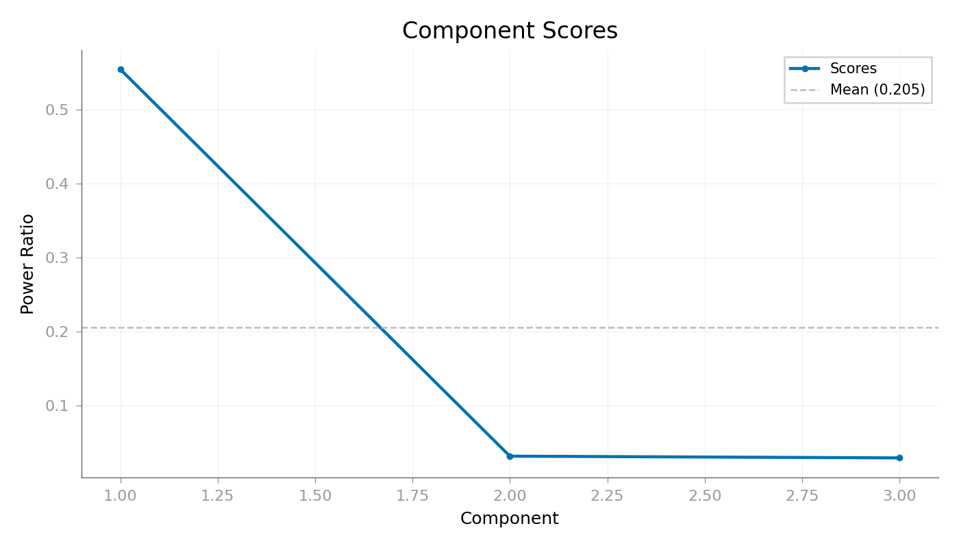
# This plot shows the "Bias Ratio" for each component.
# Expectation: The first component (Comp 0) should have a much
# higher score than the rest.
# This indicates that Comp 0 is highly reproducible (signal),
# while others are noise.
plot_component_score_curve(dss_evoked, mode="ratio", show=True)
Component Scores
--- Synthetic: Trial Average Bias ---
/home/runner/work/mne-denoise/mne-denoise/mne_denoise/dss/linear.py:496: RuntimeWarning: Epochs are not baseline corrected, covariance matrix may be inaccurate
  baseline_cov = mne.compute_covariance(inst, method=method, **kws)
/home/runner/work/mne-denoise/mne-denoise/mne_denoise/dss/linear.py:498: RuntimeWarning: Epochs are not baseline corrected, covariance matrix may be inaccurate
  biased_cov = mne.compute_covariance(biased_inst, method=method, **kws)

<Figure size 1400x800 with 1 Axes>

Component Time Series#

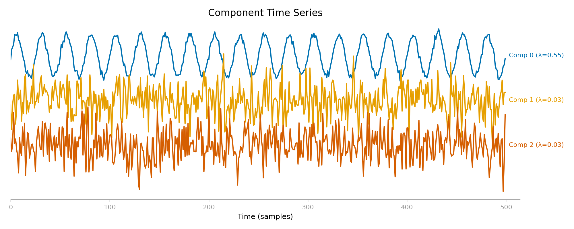
We view the time courses of the first 5 components. Expectation: Comp 0 should look like a clean 10 Hz sine wave. Expectation: Comp 1-4 should look like noise or the 50 Hz interference.

plot_component_time_series(dss_evoked, data=epochs, n_components=3, show=True)
Component Time Series
<Figure size 2000x800 with 1 Axes>

Spatial Patterns#

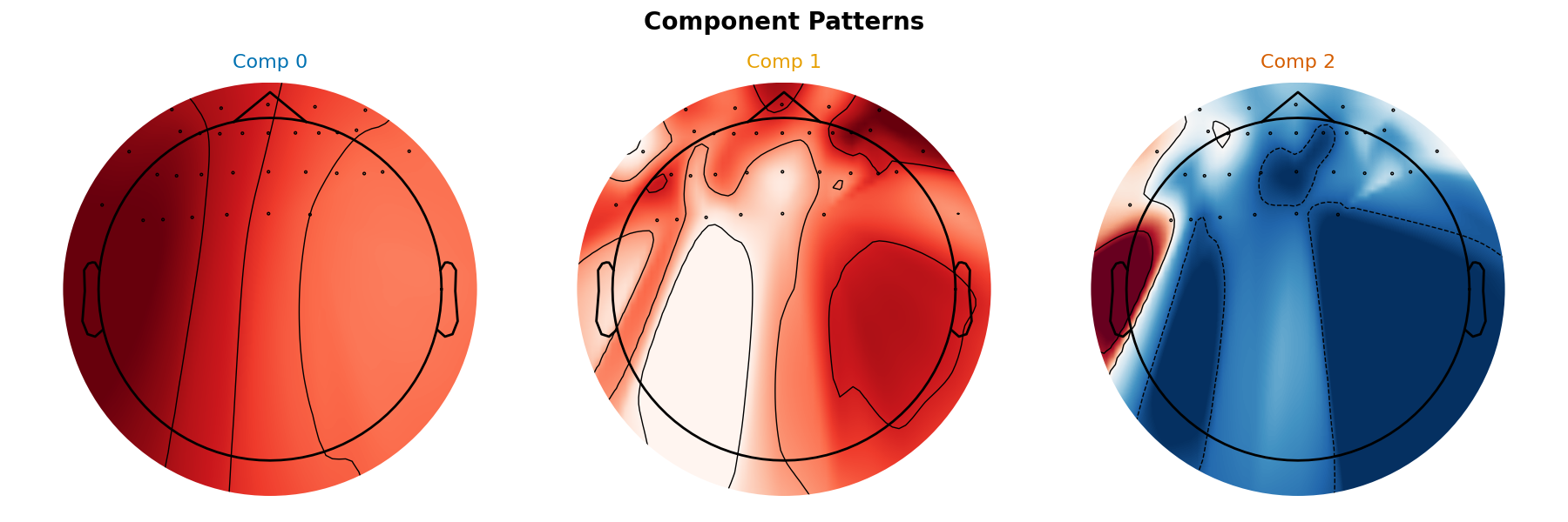
The “Spatial Pattern” (or topomap) shows how the component maps onto the sensors.

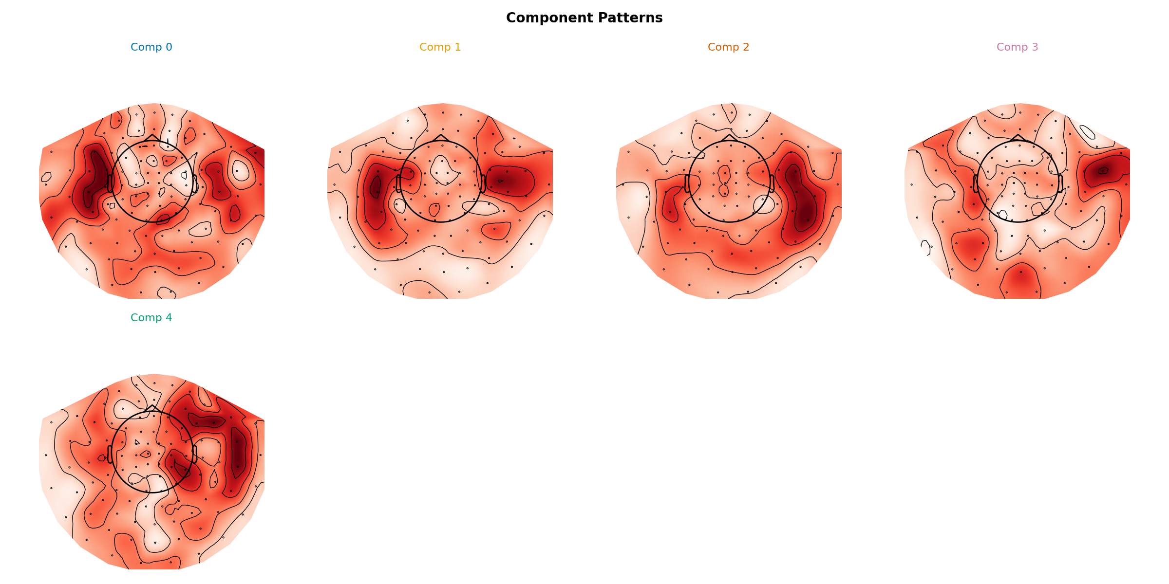
Interpretation: Colors: Red/Blue indicate opposite polarity. Strong colors mean the component is strongly present on those sensors. Dots: These represent the 32 electrodes of the ‘standard_1020’ montage. Comp 0: Shows a smooth dipolar field (the “Left-ish” pattern we simulated). Comp 1+: Often look “speckled” or messy, indicating they capture noise.

Note: Since the data is synthetic, the sensor locations are idealized.

plot_component_patterns(
    dss_evoked,
    info=epochs.info,
    picks=epochs_picks,
    n_components=3,
    show=True,
)
Component Patterns, Comp 0, Comp 1, Comp 2
<Figure size 1800x600 with 3 Axes>

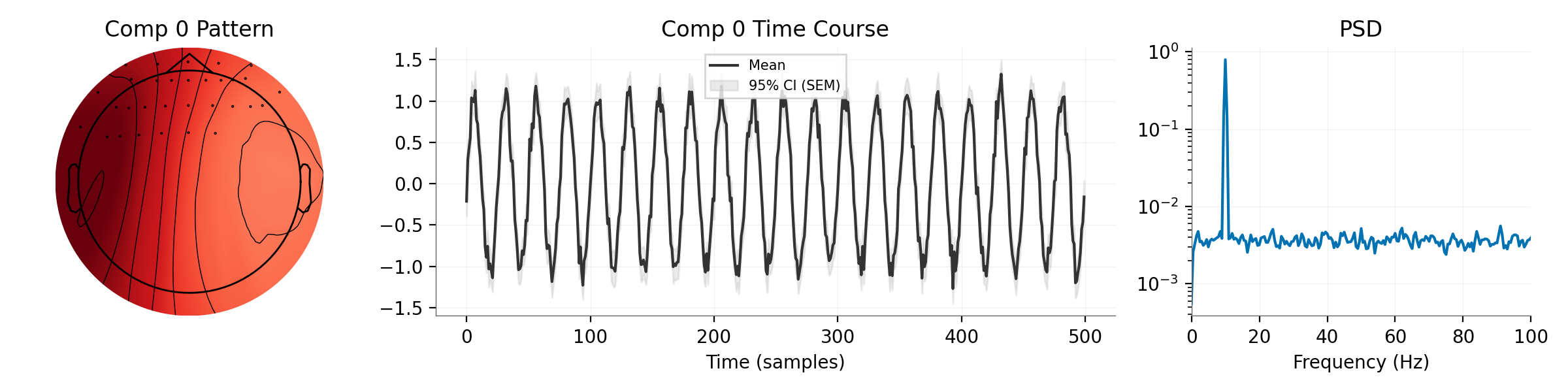
Component Summary#

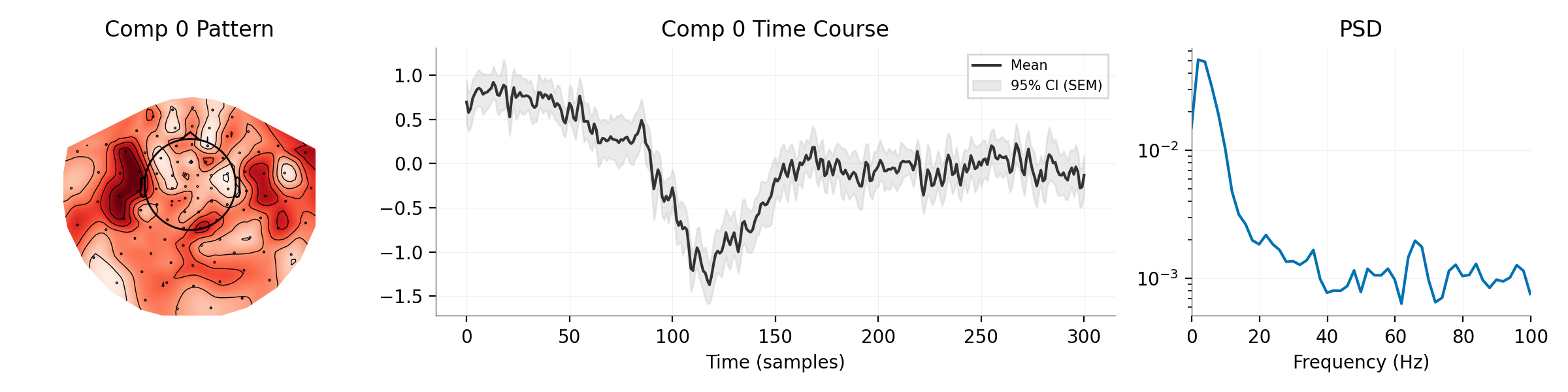
A dashboard for detailed inspection of Comp 0.

plot_component_summary(
    dss_evoked,
    data=epochs,
    info=epochs.info,
    picks=epochs_picks,
    n_components=[0],
    show=True,
)
Comp 0 Pattern, Comp 0 Time Course, PSD
<Figure size 2400x600 with 3 Axes>

Denoising Comparison#

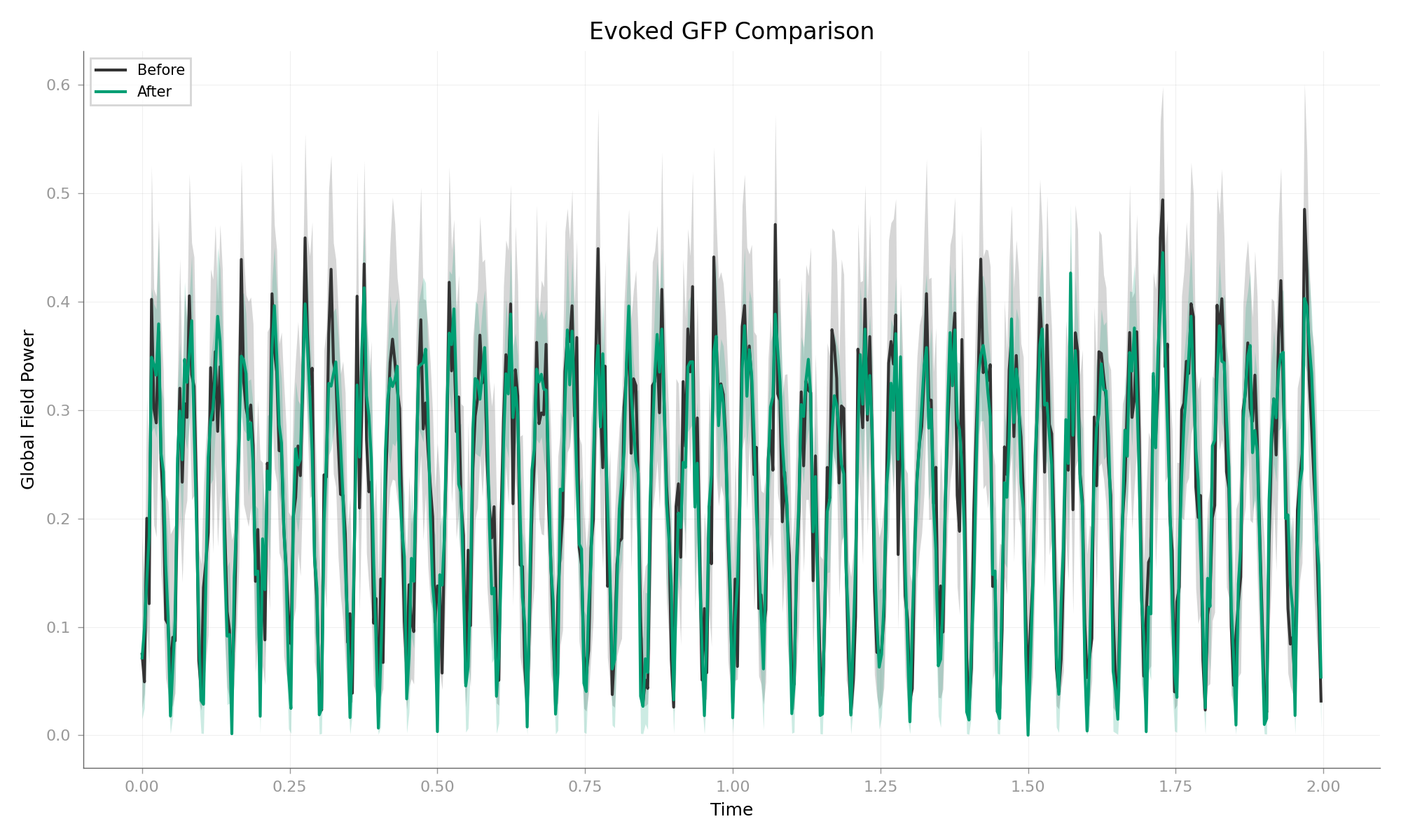
We reconstruct the data using ONLY the first component (the “Signal”). This removes the 50Hz interference and white noise.

print("Reconstructing data from first component...")
sources = dss_evoked.transform(epochs)
# To reconstruct using only specific components, we zero out the others
sources[:, 1:, :] = 0
epochs_denoised = dss_evoked.inverse_transform(sources)
epochs_denoised = mne.EpochsArray(epochs_denoised, info)

# Plot Original vs Denoised Evoked Response
# Expectation: The "Denoised" trace should have smaller confidence intervals
# because the variable noise has been removed.
plot_evoked_gfp_comparison(epochs, epochs_denoised, times=epochs.times, show=True)
Evoked GFP Comparison
Reconstructing data from first component...
Not setting metadata
50 matching events found
No baseline correction applied
0 projection items activated

<Figure size 2000x1200 with 1 Axes>

Synthetic B: Bandpass Bias#

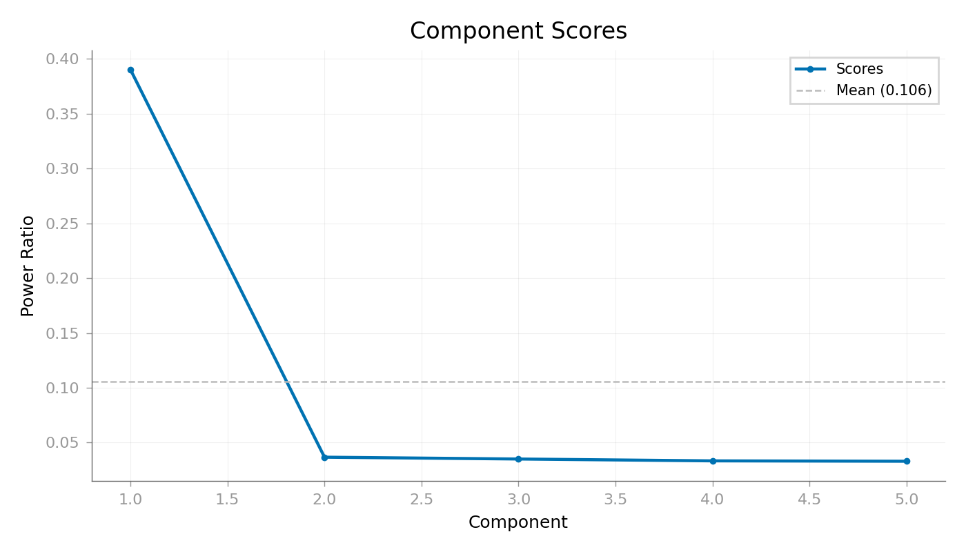
Goal: Isolate the Oscillatory (50Hz) component. Note: This component cancels out in the trial average! But DSS can find it by maximizing 50Hz power. Bias: Maximize power in 48-52 Hz band.

print("\n--- Synthetic: Bandpass Bias (50Hz) ---")
bias_bp = BandpassBias(freq_band=(48, 52), sfreq=sfreq)
dss_osc = DSS(n_components=5, bias=bias_bp)
# For Bandpass, we often treat data as continuous (Raw),
# but Epochs work too (concatenated).
dss_osc.fit(epochs)

# Visualize
# Score Curve
plot_component_score_curve(dss_osc, mode="ratio", show=True)
Component Scores
--- Synthetic: Bandpass Bias (50Hz) ---
/home/runner/work/mne-denoise/mne-denoise/mne_denoise/dss/linear.py:496: RuntimeWarning: Epochs are not baseline corrected, covariance matrix may be inaccurate
  baseline_cov = mne.compute_covariance(inst, method=method, **kws)
/home/runner/work/mne-denoise/mne-denoise/mne_denoise/dss/linear.py:498: RuntimeWarning: Epochs are not baseline corrected, covariance matrix may be inaccurate
  biased_cov = mne.compute_covariance(biased_inst, method=method, **kws)

<Figure size 1400x800 with 1 Axes>

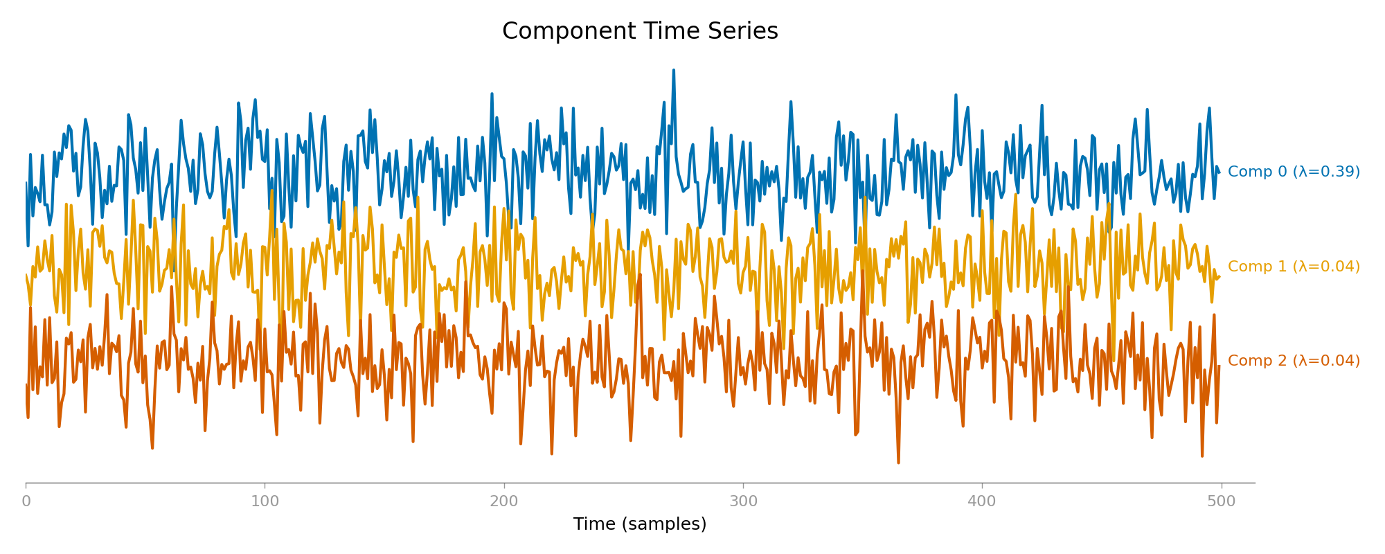
Component Time Series Expectation: Comp 0 should look like a bursty/clean 50Hz oscillation. Note: Unlike Evoked, these are not phase-locked, so peaks don’t align across trials.

plot_component_time_series(dss_osc, data=epochs, n_components=3, show=True)
Component Time Series
<Figure size 2000x800 with 1 Axes>

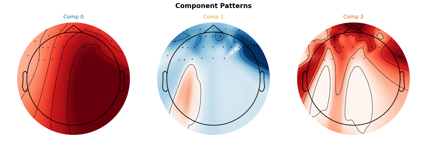
Spatial Patterns Expectation: Comp 0 should show the “Right-ish” field pattern. Note: This topography is distinct from the Evoked signal, showing how DSS separates sources spatially.

plot_component_patterns(
    dss_osc,
    info=epochs.info,
    picks=epochs_picks,
    n_components=3,
    show=True,
)
Component Patterns, Comp 0, Comp 1, Comp 2
<Figure size 1800x600 with 3 Axes>

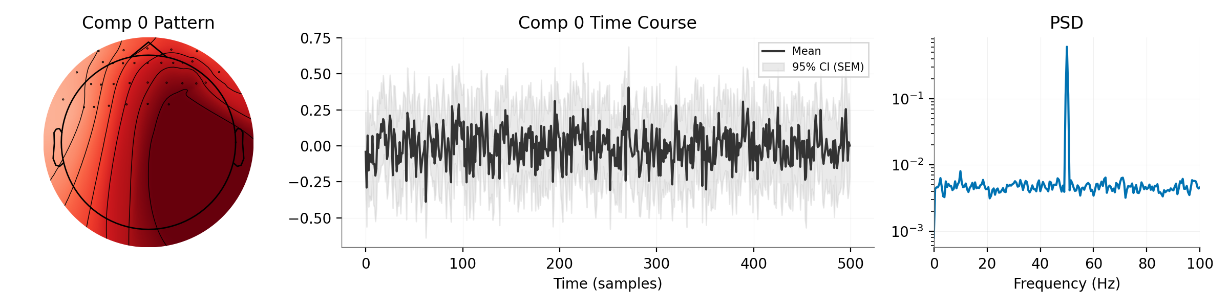
Component Summary Expectation: PSD should show a very sharp peak at 50 Hz.

plot_component_summary(
    dss_osc,
    data=epochs,
    info=epochs.info,
    picks=epochs_picks,
    n_components=[0],
    show=True,
)
Comp 0 Pattern, Comp 0 Time Course, PSD
<Figure size 2400x600 with 3 Axes>

Denoising Comparison#

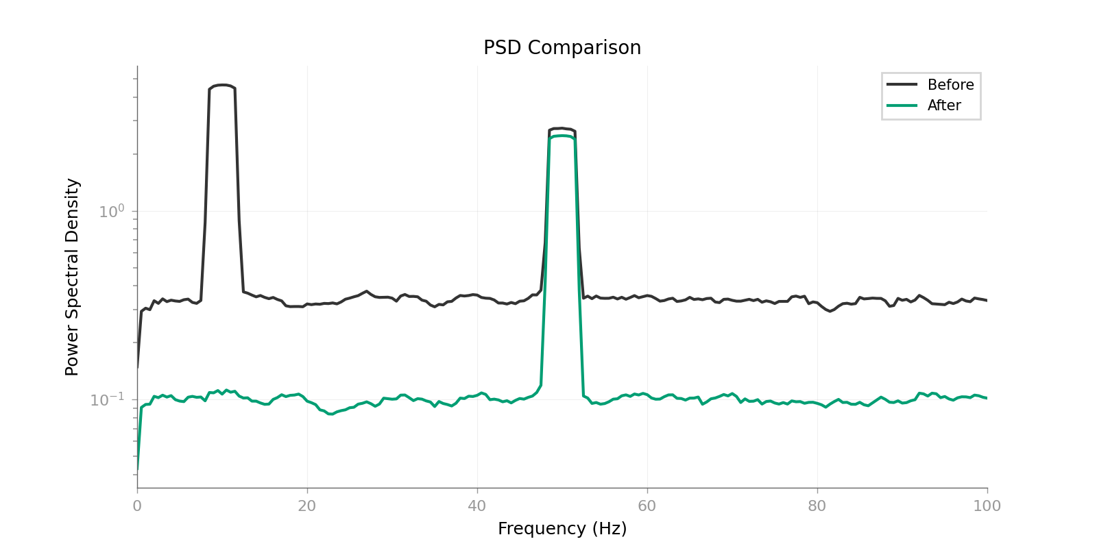
Reconstruct data using the oscillator component.

print("Reconstructing data from oscillatory component...")
# We concatenate epochs for continuous reconstruction if desired, or keep as epochs
# Here we keep as epochs to use plot_psd_comparison
sources = dss_osc.transform(epochs)
sources[:, 1:, :] = 0
epochs_osc = dss_osc.inverse_transform(sources)
epochs_osc = mne.EpochsArray(epochs_osc, info)

# Plot PSD Comparison
# Expectation: The "Denoised" signal should have a massive peak at 50 Hz
# and very little power elsewhere (noise suppressed).
plot_psd_comparison(epochs, epochs_osc, show=True, fmax=100)
PSD Comparison
Reconstructing data from oscillatory component...
Not setting metadata
50 matching events found
No baseline correction applied
0 projection items activated
    Using multitaper spectrum estimation with 7 DPSS windows
    Using multitaper spectrum estimation with 7 DPSS windows

<Figure size 1600x800 with 1 Axes>

Part 2: Real Data (MNE Sample)#

We load real MEG data and perform the same two tasks as above: recover the auditory evoked response with a trial-average bias and recover background alpha rhythm with a bandpass bias.

print("\nLoading MNE Sample data...")
# Ensure MNE_DATA directory exists
home = os.path.expanduser("~")
mne_data_path = os.path.join(home, "mne_data")
if not os.path.exists(mne_data_path):
    with contextlib.suppress(OSError):
        os.makedirs(mne_data_path)

data_path = sample.data_path()
raw_fname = data_path / "MEG" / "sample" / "sample_audvis_raw.fif"
event_fname = data_path / "MEG" / "sample" / "sample_audvis_raw-eve.fif"

raw = mne.io.read_raw_fif(raw_fname, preload=True, verbose=False)
raw.pick_types(meg="grad", eeg=False, eog=False, stim=False).crop(0, 60)
raw_picks = np.arange(len(raw.ch_names))
print(f"Data: {len(raw.ch_names)} Gradiometers, 60s duration")
Loading MNE Sample data...
Using default location ~/mne_data for sample...
Fetching 1 file for the sample dataset ...
Downloading file 'MNE-sample-data-processed.tar.gz' from 'https://osf.io/download/86qa2?version=6' to '/tmp/mne-denoise-home/mne_data'.

  0%|                                              | 0.00/1.65G [00:00<?, ?B/s]
  0%|                                     | 2.80M/1.65G [00:00<00:58, 28.0MB/s]
  1%|▏                                    | 10.2M/1.65G [00:00<00:29, 55.2MB/s]
  1%|▍                                    | 17.7M/1.65G [00:00<00:25, 64.2MB/s]
  2%|▌                                    | 25.2M/1.65G [00:00<00:23, 68.3MB/s]
  2%|▋                                    | 32.8M/1.65G [00:00<00:22, 71.0MB/s]
  2%|▉                                    | 40.5M/1.65G [00:00<00:22, 73.2MB/s]
  3%|█                                    | 48.2M/1.65G [00:00<00:21, 74.3MB/s]
  3%|█▎                                   | 55.9M/1.65G [00:00<00:21, 75.4MB/s]
  4%|█▍                                   | 63.5M/1.65G [00:00<00:21, 75.6MB/s]
  4%|█▌                                   | 71.1M/1.65G [00:01<00:20, 75.7MB/s]
  5%|█▊                                   | 78.7M/1.65G [00:01<00:20, 75.8MB/s]
  5%|█▉                                   | 86.4M/1.65G [00:01<00:20, 76.1MB/s]
  6%|██                                   | 94.2M/1.65G [00:01<00:20, 76.6MB/s]
  6%|██▎                                   | 102M/1.65G [00:01<00:20, 76.3MB/s]
  7%|██▌                                   | 110M/1.65G [00:01<00:20, 76.5MB/s]
  7%|██▋                                   | 117M/1.65G [00:01<00:20, 76.4MB/s]
  8%|██▊                                   | 125M/1.65G [00:01<00:20, 75.6MB/s]
  8%|███                                   | 133M/1.65G [00:01<00:19, 76.2MB/s]
  8%|███▏                                  | 140M/1.65G [00:01<00:19, 76.4MB/s]
  9%|███▍                                  | 148M/1.65G [00:02<00:19, 76.7MB/s]
  9%|███▌                                  | 156M/1.65G [00:02<00:19, 77.0MB/s]
 10%|███▊                                  | 163M/1.65G [00:02<00:19, 77.0MB/s]
 10%|███▉                                  | 171M/1.65G [00:02<00:19, 77.1MB/s]
 11%|████                                  | 179M/1.65G [00:02<00:19, 77.0MB/s]
 11%|████▎                                 | 187M/1.65G [00:02<00:19, 76.7MB/s]
 12%|████▍                                 | 194M/1.65G [00:02<00:18, 76.9MB/s]
 12%|████▋                                 | 202M/1.65G [00:02<00:19, 75.6MB/s]
 13%|████▊                                 | 210M/1.65G [00:02<00:19, 75.4MB/s]
 13%|████▉                                 | 217M/1.65G [00:02<00:18, 75.8MB/s]
 14%|█████▏                                | 225M/1.65G [00:03<00:18, 76.2MB/s]
 14%|█████▎                                | 233M/1.65G [00:03<00:18, 76.0MB/s]
 15%|█████▌                                | 240M/1.65G [00:03<00:18, 76.3MB/s]
 15%|█████▋                                | 248M/1.65G [00:03<00:18, 76.4MB/s]
 15%|█████▉                                | 256M/1.65G [00:03<00:18, 76.7MB/s]
 16%|██████                                | 263M/1.65G [00:03<00:18, 76.9MB/s]
 16%|██████▏                               | 271M/1.65G [00:03<00:17, 77.1MB/s]
 17%|██████▍                               | 279M/1.65G [00:03<00:17, 76.8MB/s]
 17%|██████▌                               | 287M/1.65G [00:03<00:18, 74.6MB/s]
 18%|██████▊                               | 294M/1.65G [00:03<00:18, 74.9MB/s]
 18%|██████▉                               | 302M/1.65G [00:04<00:17, 75.4MB/s]
 19%|███████                               | 310M/1.65G [00:04<00:17, 75.9MB/s]
 19%|███████▎                              | 317M/1.65G [00:04<00:17, 76.2MB/s]
 20%|███████▍                              | 325M/1.65G [00:04<00:17, 76.4MB/s]
 20%|███████▋                              | 333M/1.65G [00:04<00:17, 76.7MB/s]
 21%|███████▊                              | 340M/1.65G [00:04<00:17, 77.0MB/s]
 21%|████████                              | 348M/1.65G [00:04<00:16, 77.1MB/s]
 22%|████████▏                             | 356M/1.65G [00:04<00:16, 76.9MB/s]
 22%|████████▎                             | 364M/1.65G [00:04<00:16, 76.9MB/s]
 22%|████████▌                             | 371M/1.65G [00:04<00:16, 76.9MB/s]
 23%|████████▋                             | 379M/1.65G [00:05<00:16, 76.8MB/s]
 23%|████████▉                             | 387M/1.65G [00:05<00:18, 68.4MB/s]
 24%|█████████                             | 394M/1.65G [00:05<00:19, 65.9MB/s]
 24%|█████████▏                            | 401M/1.65G [00:05<00:18, 68.6MB/s]
 25%|█████████▍                            | 409M/1.65G [00:05<00:17, 71.1MB/s]
 25%|█████████▌                            | 417M/1.65G [00:05<00:16, 72.8MB/s]
 26%|█████████▊                            | 424M/1.65G [00:05<00:16, 74.1MB/s]
 26%|█████████▉                            | 432M/1.65G [00:05<00:16, 74.8MB/s]
 27%|██████████                            | 440M/1.65G [00:05<00:16, 75.5MB/s]
 27%|██████████▎                           | 447M/1.65G [00:05<00:15, 75.8MB/s]
 28%|██████████▍                           | 455M/1.65G [00:06<00:15, 75.9MB/s]
 28%|██████████▋                           | 463M/1.65G [00:06<00:15, 76.2MB/s]
 28%|██████████▊                           | 470M/1.65G [00:06<00:15, 76.2MB/s]
 29%|██████████▉                           | 478M/1.65G [00:06<00:15, 76.5MB/s]
 29%|███████████▏                          | 486M/1.65G [00:06<00:15, 76.7MB/s]
 30%|███████████▎                          | 494M/1.65G [00:06<00:15, 76.9MB/s]
 30%|███████████▌                          | 501M/1.65G [00:06<00:15, 76.7MB/s]
 31%|███████████▋                          | 509M/1.65G [00:06<00:15, 75.6MB/s]
 31%|███████████▉                          | 517M/1.65G [00:06<00:15, 75.7MB/s]
 32%|████████████                          | 524M/1.65G [00:06<00:14, 76.2MB/s]
 32%|████████████▏                         | 532M/1.65G [00:07<00:14, 76.2MB/s]
 33%|████████████▍                         | 540M/1.65G [00:07<00:14, 76.3MB/s]
 33%|████████████▌                         | 547M/1.65G [00:07<00:14, 76.5MB/s]
 34%|████████████▊                         | 555M/1.65G [00:07<00:14, 76.6MB/s]
 34%|████████████▉                         | 563M/1.65G [00:07<00:14, 76.7MB/s]
 35%|█████████████                         | 570M/1.65G [00:07<00:14, 76.8MB/s]
 35%|█████████████▎                        | 578M/1.65G [00:07<00:14, 76.6MB/s]
 35%|█████████████▍                        | 586M/1.65G [00:07<00:13, 76.8MB/s]
 36%|█████████████▋                        | 594M/1.65G [00:07<00:13, 77.2MB/s]
 36%|█████████████▊                        | 601M/1.65G [00:07<00:13, 77.3MB/s]
 37%|██████████████                        | 609M/1.65G [00:08<00:13, 77.0MB/s]
 37%|██████████████▏                       | 617M/1.65G [00:08<00:13, 77.1MB/s]
 38%|██████████████▎                       | 625M/1.65G [00:08<00:13, 77.3MB/s]
 38%|██████████████▌                       | 632M/1.65G [00:08<00:13, 77.3MB/s]
 39%|██████████████▋                       | 640M/1.65G [00:08<00:13, 77.3MB/s]
 39%|██████████████▉                       | 648M/1.65G [00:08<00:12, 77.6MB/s]
 40%|███████████████                       | 656M/1.65G [00:08<00:12, 77.5MB/s]
 40%|███████████████▎                      | 663M/1.65G [00:08<00:12, 77.7MB/s]
 41%|███████████████▍                      | 671M/1.65G [00:08<00:13, 74.3MB/s]
 41%|███████████████▌                      | 679M/1.65G [00:09<00:12, 75.1MB/s]
 42%|███████████████▊                      | 687M/1.65G [00:09<00:12, 75.8MB/s]
 42%|███████████████▉                      | 694M/1.65G [00:09<00:12, 76.3MB/s]
 42%|████████████████▏                     | 702M/1.65G [00:09<00:12, 76.8MB/s]
 43%|████████████████▎                     | 710M/1.65G [00:09<00:12, 77.0MB/s]
 43%|████████████████▌                     | 718M/1.65G [00:09<00:12, 77.3MB/s]
 44%|████████████████▋                     | 725M/1.65G [00:09<00:12, 77.2MB/s]
 44%|████████████████▊                     | 733M/1.65G [00:09<00:11, 77.1MB/s]
 45%|█████████████████                     | 741M/1.65G [00:09<00:11, 76.9MB/s]
 45%|█████████████████▏                    | 749M/1.65G [00:09<00:11, 77.2MB/s]
 46%|█████████████████▍                    | 756M/1.65G [00:10<00:11, 77.0MB/s]
 46%|█████████████████▌                    | 764M/1.65G [00:10<00:11, 77.3MB/s]
 47%|█████████████████▋                    | 772M/1.65G [00:10<00:11, 77.4MB/s]
 47%|█████████████████▉                    | 780M/1.65G [00:10<00:11, 77.4MB/s]
 48%|██████████████████                    | 788M/1.65G [00:10<00:11, 77.4MB/s]
 48%|██████████████████▎                   | 795M/1.65G [00:10<00:11, 77.6MB/s]
 49%|██████████████████▍                   | 803M/1.65G [00:10<00:10, 77.5MB/s]
 49%|██████████████████▋                   | 811M/1.65G [00:10<00:10, 76.8MB/s]
 50%|██████████████████▊                   | 819M/1.65G [00:10<00:10, 76.8MB/s]
 50%|███████████████████                   | 826M/1.65G [00:10<00:10, 77.4MB/s]
 50%|███████████████████▏                  | 834M/1.65G [00:11<00:10, 77.4MB/s]
 51%|███████████████████▎                  | 842M/1.65G [00:11<00:10, 77.7MB/s]
 51%|███████████████████▌                  | 850M/1.65G [00:11<00:10, 77.8MB/s]
 52%|███████████████████▋                  | 858M/1.65G [00:11<00:10, 76.4MB/s]
 52%|███████████████████▉                  | 865M/1.65G [00:11<00:10, 75.9MB/s]
 53%|████████████████████                  | 873M/1.65G [00:11<00:10, 75.2MB/s]
 53%|████████████████████▏                 | 880M/1.65G [00:11<00:10, 72.6MB/s]
 54%|████████████████████▍                 | 888M/1.65G [00:11<00:10, 73.8MB/s]
 54%|████████████████████▌                 | 896M/1.65G [00:11<00:10, 74.8MB/s]
 55%|████████████████████▊                 | 903M/1.65G [00:11<00:09, 75.5MB/s]
 55%|████████████████████▉                 | 911M/1.65G [00:12<00:09, 76.1MB/s]
 56%|█████████████████████▏                | 919M/1.65G [00:12<00:09, 76.6MB/s]
 56%|█████████████████████▎                | 927M/1.65G [00:12<00:09, 75.1MB/s]
 57%|█████████████████████▍                | 934M/1.65G [00:12<00:10, 66.8MB/s]
 57%|█████████████████████▋                | 941M/1.65G [00:12<00:10, 67.5MB/s]
 57%|█████████████████████▊                | 949M/1.65G [00:12<00:10, 70.3MB/s]
 58%|█████████████████████▉                | 956M/1.65G [00:12<00:09, 71.7MB/s]
 58%|██████████████████████▏               | 964M/1.65G [00:12<00:09, 72.2MB/s]
 59%|██████████████████████▎               | 971M/1.65G [00:12<00:09, 73.4MB/s]
 59%|██████████████████████▌               | 979M/1.65G [00:12<00:09, 74.1MB/s]
 60%|██████████████████████▋               | 986M/1.65G [00:13<00:09, 73.9MB/s]
 60%|██████████████████████▊               | 994M/1.65G [00:13<00:08, 74.5MB/s]
 61%|██████████████████████▍              | 1.00G/1.65G [00:13<00:08, 74.8MB/s]
 61%|██████████████████████▌              | 1.01G/1.65G [00:13<00:08, 75.2MB/s]
 62%|██████████████████████▊              | 1.02G/1.65G [00:13<00:08, 75.4MB/s]
 62%|██████████████████████▉              | 1.02G/1.65G [00:13<00:08, 75.7MB/s]
 62%|███████████████████████              | 1.03G/1.65G [00:13<00:08, 76.0MB/s]
 63%|███████████████████████▎             | 1.04G/1.65G [00:13<00:08, 76.5MB/s]
 63%|███████████████████████▍             | 1.05G/1.65G [00:13<00:08, 74.9MB/s]
 64%|███████████████████████▌             | 1.06G/1.65G [00:13<00:07, 75.5MB/s]
 64%|███████████████████████▊             | 1.06G/1.65G [00:14<00:07, 75.9MB/s]
 65%|███████████████████████▉             | 1.07G/1.65G [00:14<00:07, 76.7MB/s]
 65%|████████████████████████▏            | 1.08G/1.65G [00:14<00:07, 76.8MB/s]
 66%|████████████████████████▎            | 1.09G/1.65G [00:14<00:07, 77.0MB/s]
 66%|████████████████████████▍            | 1.09G/1.65G [00:14<00:07, 77.1MB/s]
 67%|████████████████████████▋            | 1.10G/1.65G [00:14<00:07, 77.0MB/s]
 67%|████████████████████████▊            | 1.11G/1.65G [00:14<00:07, 76.4MB/s]
 68%|█████████████████████████            | 1.12G/1.65G [00:14<00:07, 76.3MB/s]
 68%|█████████████████████████▏           | 1.12G/1.65G [00:14<00:06, 76.4MB/s]
 69%|█████████████████████████▎           | 1.13G/1.65G [00:15<00:06, 76.6MB/s]
 69%|█████████████████████████▌           | 1.14G/1.65G [00:15<00:06, 76.8MB/s]
 69%|█████████████████████████▋           | 1.15G/1.65G [00:15<00:06, 76.6MB/s]
 70%|█████████████████████████▊           | 1.16G/1.65G [00:15<00:06, 76.6MB/s]
 70%|██████████████████████████           | 1.16G/1.65G [00:15<00:06, 76.7MB/s]
 71%|██████████████████████████▏          | 1.17G/1.65G [00:15<00:06, 76.7MB/s]
 71%|██████████████████████████▍          | 1.18G/1.65G [00:15<00:06, 76.7MB/s]
 72%|██████████████████████████▌          | 1.19G/1.65G [00:15<00:06, 76.6MB/s]
 72%|██████████████████████████▋          | 1.19G/1.65G [00:15<00:06, 76.4MB/s]
 73%|██████████████████████████▉          | 1.20G/1.65G [00:15<00:05, 76.5MB/s]
 73%|███████████████████████████          | 1.21G/1.65G [00:16<00:05, 76.7MB/s]
 74%|███████████████████████████▏         | 1.22G/1.65G [00:16<00:05, 76.7MB/s]
 74%|███████████████████████████▍         | 1.22G/1.65G [00:16<00:05, 76.7MB/s]
 75%|███████████████████████████▌         | 1.23G/1.65G [00:16<00:05, 76.6MB/s]
 75%|███████████████████████████▊         | 1.24G/1.65G [00:16<00:05, 76.7MB/s]
 75%|███████████████████████████▉         | 1.25G/1.65G [00:16<00:05, 76.8MB/s]
 76%|████████████████████████████         | 1.26G/1.65G [00:16<00:05, 76.8MB/s]
 76%|████████████████████████████▎        | 1.26G/1.65G [00:16<00:05, 76.5MB/s]
 77%|████████████████████████████▍        | 1.27G/1.65G [00:16<00:05, 76.0MB/s]
 77%|████████████████████████████▌        | 1.28G/1.65G [00:16<00:04, 76.1MB/s]
 78%|████████████████████████████▊        | 1.29G/1.65G [00:17<00:04, 76.3MB/s]
 78%|████████████████████████████▉        | 1.29G/1.65G [00:17<00:04, 76.4MB/s]
 79%|█████████████████████████████▏       | 1.30G/1.65G [00:17<00:04, 76.5MB/s]
 79%|█████████████████████████████▎       | 1.31G/1.65G [00:17<00:04, 76.6MB/s]
 80%|█████████████████████████████▍       | 1.32G/1.65G [00:17<00:04, 76.8MB/s]
 80%|█████████████████████████████▋       | 1.32G/1.65G [00:17<00:04, 76.3MB/s]
 81%|█████████████████████████████▊       | 1.33G/1.65G [00:17<00:04, 76.4MB/s]
 81%|█████████████████████████████▉       | 1.34G/1.65G [00:17<00:04, 76.2MB/s]
 82%|██████████████████████████████▏      | 1.35G/1.65G [00:17<00:04, 76.2MB/s]
 82%|██████████████████████████████▎      | 1.35G/1.65G [00:17<00:03, 75.5MB/s]
 82%|██████████████████████████████▌      | 1.36G/1.65G [00:18<00:03, 75.1MB/s]
 83%|██████████████████████████████▋      | 1.37G/1.65G [00:18<00:03, 75.4MB/s]
 83%|██████████████████████████████▊      | 1.38G/1.65G [00:18<00:03, 75.7MB/s]
 84%|███████████████████████████████      | 1.39G/1.65G [00:18<00:03, 75.9MB/s]
 84%|███████████████████████████████▏     | 1.39G/1.65G [00:18<00:03, 76.3MB/s]
 85%|███████████████████████████████▎     | 1.40G/1.65G [00:18<00:03, 76.4MB/s]
 85%|███████████████████████████████▌     | 1.41G/1.65G [00:18<00:03, 76.5MB/s]
 86%|███████████████████████████████▋     | 1.42G/1.65G [00:18<00:03, 76.6MB/s]
 86%|███████████████████████████████▊     | 1.42G/1.65G [00:18<00:02, 76.6MB/s]
 87%|████████████████████████████████     | 1.43G/1.65G [00:18<00:02, 76.7MB/s]
 87%|████████████████████████████████▏    | 1.44G/1.65G [00:19<00:02, 76.7MB/s]
 88%|████████████████████████████████▍    | 1.45G/1.65G [00:19<00:02, 76.3MB/s]
 88%|████████████████████████████████▌    | 1.45G/1.65G [00:19<00:02, 76.4MB/s]
 88%|████████████████████████████████▋    | 1.46G/1.65G [00:19<00:02, 76.6MB/s]
 89%|████████████████████████████████▉    | 1.47G/1.65G [00:19<00:02, 76.7MB/s]
 89%|█████████████████████████████████    | 1.48G/1.65G [00:19<00:02, 76.7MB/s]
 90%|█████████████████████████████████▏   | 1.49G/1.65G [00:19<00:02, 76.7MB/s]
 90%|█████████████████████████████████▍   | 1.49G/1.65G [00:19<00:02, 76.5MB/s]
 91%|█████████████████████████████████▌   | 1.50G/1.65G [00:19<00:01, 76.3MB/s]
 91%|█████████████████████████████████▊   | 1.51G/1.65G [00:19<00:01, 76.3MB/s]
 92%|█████████████████████████████████▉   | 1.52G/1.65G [00:20<00:01, 76.4MB/s]
 92%|██████████████████████████████████   | 1.52G/1.65G [00:20<00:01, 76.4MB/s]
 93%|██████████████████████████████████▎  | 1.53G/1.65G [00:20<00:01, 76.5MB/s]
 93%|██████████████████████████████████▍  | 1.54G/1.65G [00:20<00:01, 76.5MB/s]
 94%|██████████████████████████████████▌  | 1.55G/1.65G [00:20<00:01, 76.4MB/s]
 94%|██████████████████████████████████▊  | 1.55G/1.65G [00:20<00:01, 76.6MB/s]
 94%|██████████████████████████████████▉  | 1.56G/1.65G [00:20<00:01, 68.2MB/s]
 95%|███████████████████████████████████  | 1.57G/1.65G [00:20<00:01, 66.4MB/s]
 95%|███████████████████████████████████▎ | 1.58G/1.65G [00:20<00:01, 69.2MB/s]
 96%|███████████████████████████████████▍ | 1.58G/1.65G [00:20<00:00, 71.2MB/s]
 96%|███████████████████████████████████▌ | 1.59G/1.65G [00:21<00:00, 70.9MB/s]
 97%|███████████████████████████████████▊ | 1.60G/1.65G [00:21<00:00, 70.9MB/s]
 97%|███████████████████████████████████▉ | 1.61G/1.65G [00:21<00:00, 72.3MB/s]
 98%|████████████████████████████████████▏| 1.61G/1.65G [00:21<00:00, 73.6MB/s]
 98%|████████████████████████████████████▎| 1.62G/1.65G [00:21<00:00, 74.5MB/s]
 99%|████████████████████████████████████▍| 1.63G/1.65G [00:21<00:00, 75.2MB/s]
 99%|████████████████████████████████████▋| 1.64G/1.65G [00:21<00:00, 75.6MB/s]
 99%|████████████████████████████████████▊| 1.64G/1.65G [00:21<00:00, 76.0MB/s]
100%|████████████████████████████████████▉| 1.65G/1.65G [00:21<00:00, 76.1MB/s]
  0%|                                              | 0.00/1.65G [00:00<?, ?B/s]
100%|█████████████████████████████████████| 1.65G/1.65G [00:00<00:00, 7.85TB/s]
Untarring contents of '/tmp/mne-denoise-home/mne_data/MNE-sample-data-processed.tar.gz' to '/tmp/mne-denoise-home/mne_data'
Attempting to create new mne-python configuration file:
/tmp/tmpjuhgh_kt/.mne/mne-python.json
Could not read the /tmp/tmpjuhgh_kt/.mne/mne-python.json json file during the writing. Assuming it is empty. Got: Expecting value: line 1 column 1 (char 0)
Download complete in 49s (1576.2 MB)
NOTE: pick_types() is a legacy function. New code should use inst.pick(...).
Data: 203 Gradiometers, 60s duration

Real A: Bandpass Bias (Alpha Rhythm)#

Goal: Find Alpha (8-12 Hz) components.

print("\n--- Real: Bandpass Bias (Alpha) ---")
bias_alpha = BandpassBias(freq_band=(8, 12), sfreq=raw.info["sfreq"])
dss_alpha = DSS(n_components=5, bias=bias_alpha)
dss_alpha.fit(raw)

# Visualize
# Score Curve
plot_component_score_curve(dss_alpha, mode="ratio", show=True)
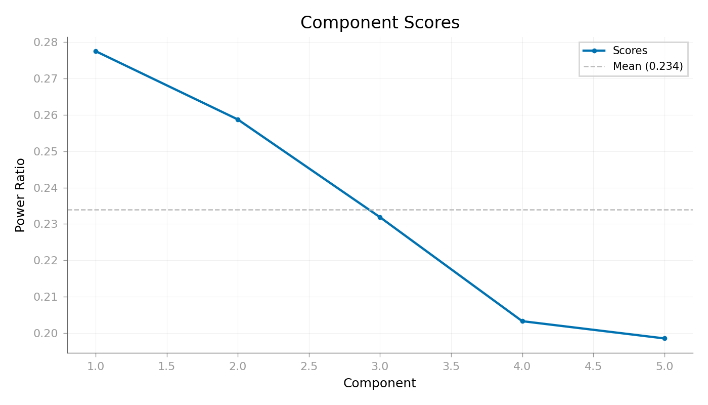
Component Scores
--- Real: Bandpass Bias (Alpha) ---

<Figure size 1400x800 with 1 Axes>

Component Time Series Expectation: Strong rhythmic activity (alpha waves) in the first component.

plot_component_time_series(dss_alpha, data=raw, n_components=5, show=True)
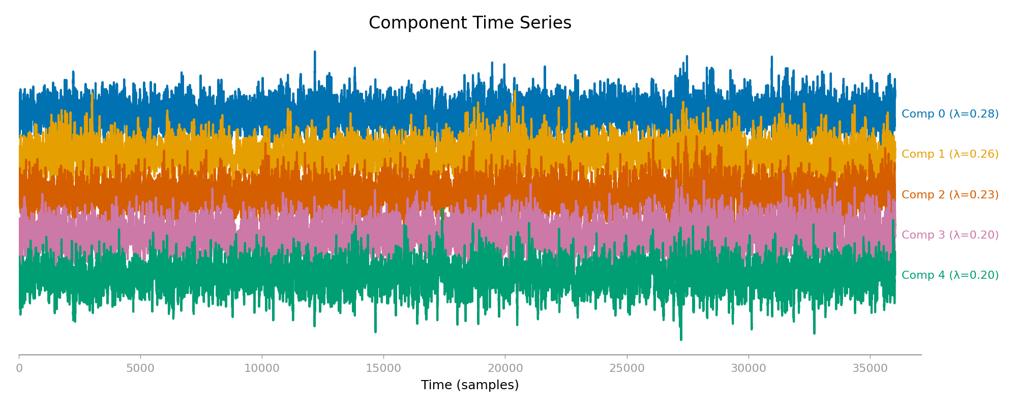
Component Time Series
<Figure size 2000x800 with 1 Axes>

Spatial Patterns Expectation: Comp 0 shows a posterior/occipital topography (visual/alpha areas). Note: The dots here represent the MEG sensors (gradiometers).

plot_component_patterns(
    dss_alpha,
    info=raw.info,
    picks=raw_picks,
    n_components=5,
    show=True,
)
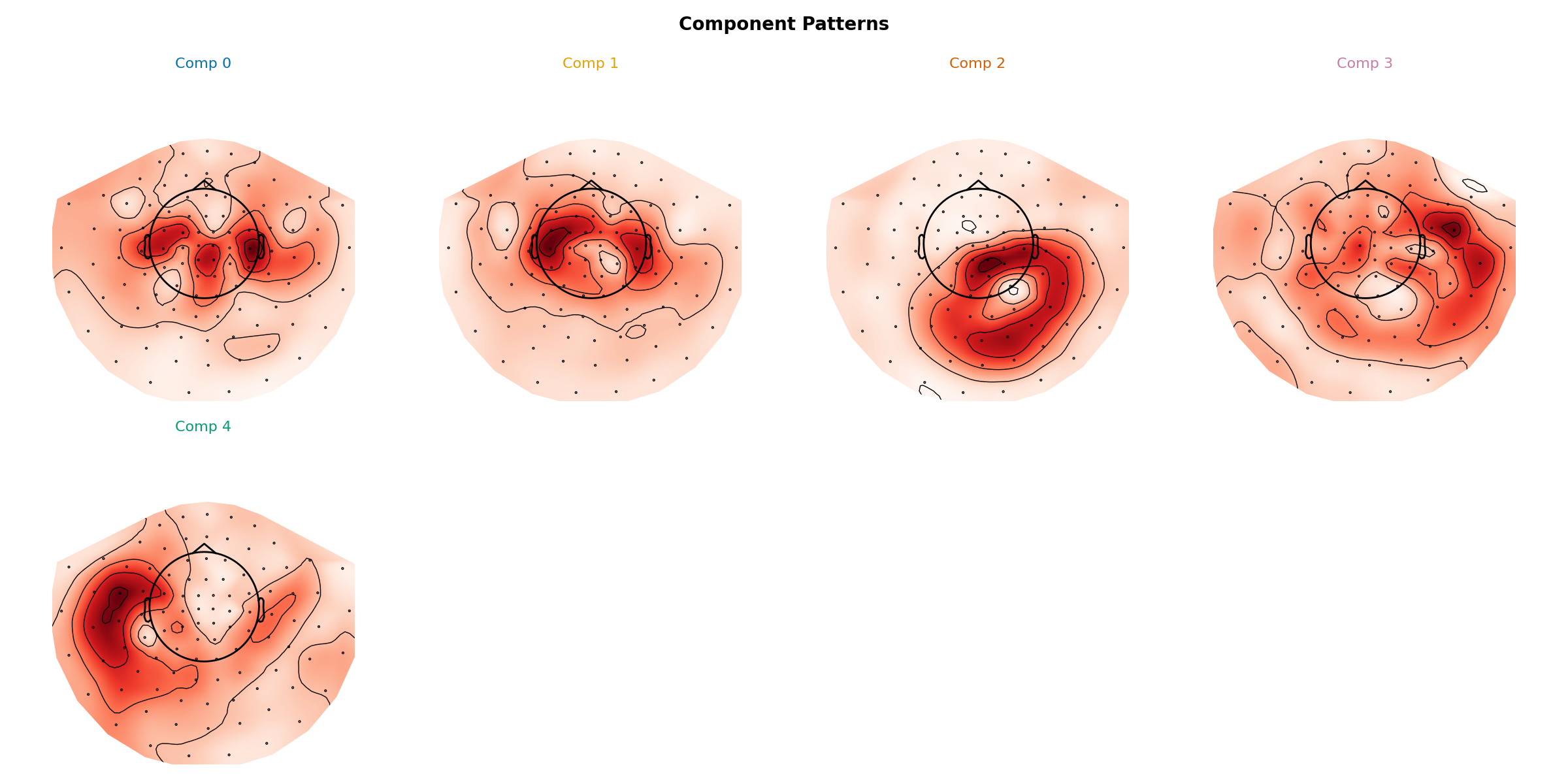
Component Patterns, Comp 0, Comp 1, Comp 2, Comp 3, Comp 4
<Figure size 2400x1200 with 8 Axes>

Component Summary Expectation: PSD peak in 8-12 Hz range.
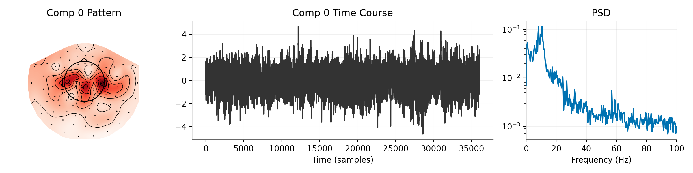
plot_component_summary(
    dss_alpha,
    data=raw,
    info=raw.info,
    picks=raw_picks,
    n_components=[0],
    show=True,
)
Comp 0 Pattern, Comp 0 Time Course, PSD
<Figure size 2400x600 with 3 Axes>

Denoising Comparison

print("Reconstructing Alpha component...")
sources_alpha = dss_alpha.transform(raw)
sources_alpha[1:, :] = 0
raw_alpha = dss_alpha.inverse_transform(sources_alpha)
raw_alpha = mne.io.RawArray(raw_alpha, raw.info)

# Compare PSDs
# Expectation: Denoised signal roughly follows original in
# alpha band but has lower noise floor.
plot_psd_comparison(raw, raw_alpha, fmax=40, show=True)
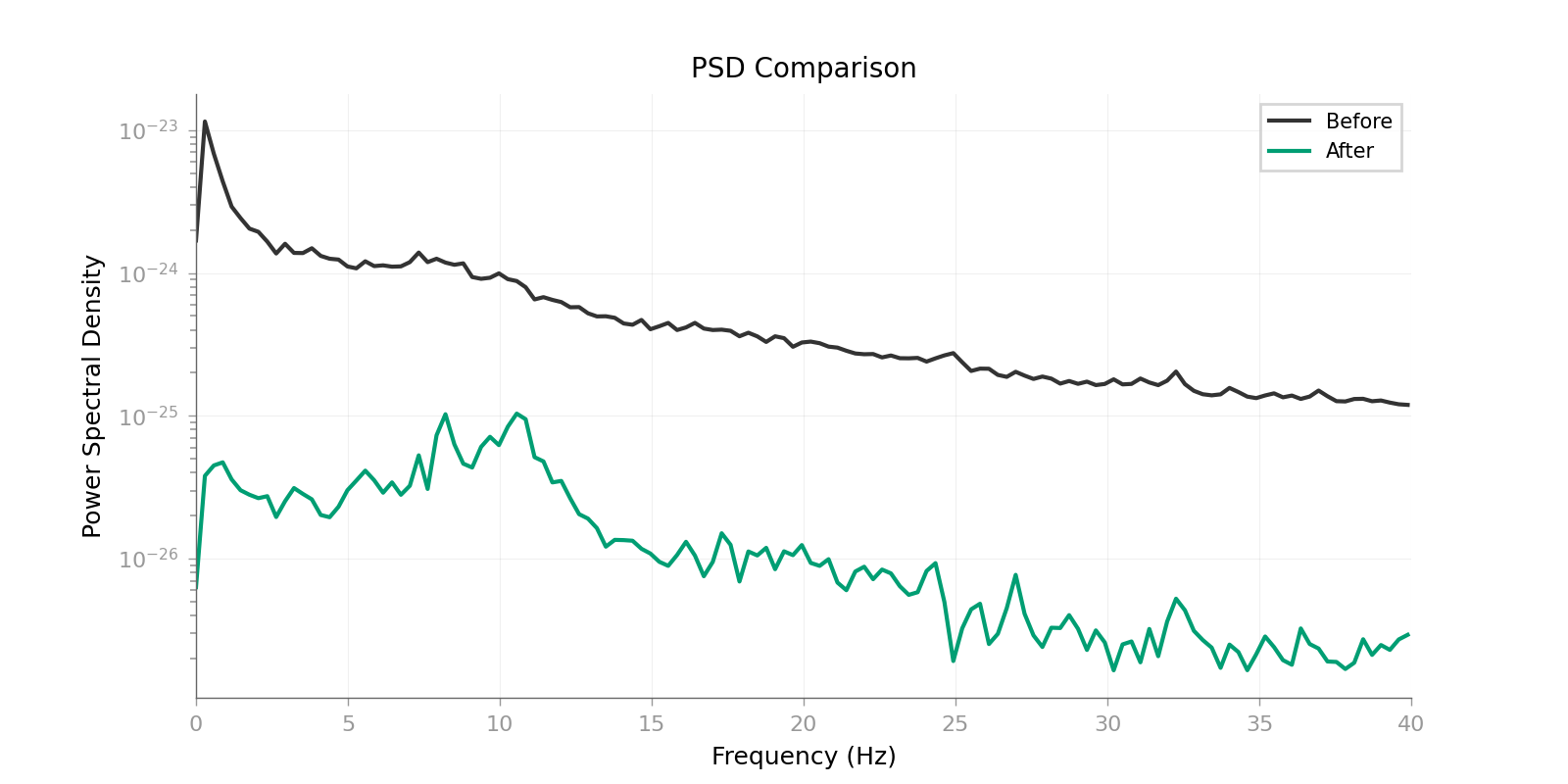
PSD Comparison
Reconstructing Alpha component...
Creating RawArray with float64 data, n_channels=203, n_times=36038
    Range : 0 ... 36037 =      0.000 ...    60.000 secs
Ready.
Effective window size : 3.410 (s)

<Figure size 1600x800 with 1 Axes>

Real B: Trial Average Bias (Auditory Evoked)#

Goal: Find the M100 auditory response. We first need to epoch the data around auditory events.

print("\n--- Real: Trial Average Bias (M100) ---")
events = mne.read_events(event_fname)
# Event ID 1 = Auditory/Left
epochs_real = mne.Epochs(
    raw,
    events,
    event_id=1,
    tmin=-0.1,
    tmax=0.4,
    baseline=(None, 0),
    preload=True,
    verbose=False,
)
print(f"Epochs extracted: {len(epochs_real)}")
epochs_real_picks = np.arange(len(epochs_real.ch_names))

dss_m100 = DSS(n_components=5, bias=AverageBias())
dss_m100.fit(epochs_real)

# Visualize
# Score Curve
plot_component_score_curve(dss_m100, mode="ratio", show=True)
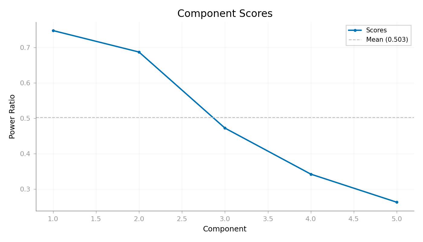
Component Scores
--- Real: Trial Average Bias (M100) ---
Epochs extracted: 20
/home/runner/work/mne-denoise/mne-denoise/mne_denoise/dss/linear.py:496: RuntimeWarning: Epochs are not baseline corrected, covariance matrix may be inaccurate
  baseline_cov = mne.compute_covariance(inst, method=method, **kws)
/home/runner/work/mne-denoise/mne-denoise/mne_denoise/dss/linear.py:498: RuntimeWarning: Epochs are not baseline corrected, covariance matrix may be inaccurate
  biased_cov = mne.compute_covariance(biased_inst, method=method, **kws)

<Figure size 1400x800 with 1 Axes>

Component Time Series Expectation: Comp 0 should show a clear evoked potential (M100) that is visible even in the stacked single trials (if SNR is good enough) or at least in the mean.

plot_component_time_series(dss_m100, data=epochs_real, n_components=5, show=True)
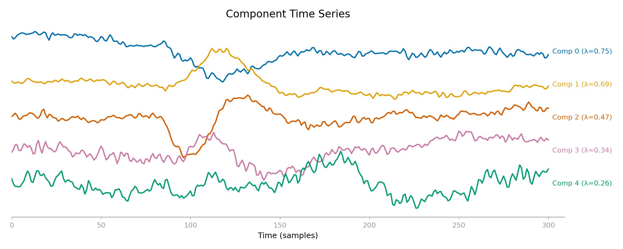
Component Time Series
<Figure size 2000x800 with 1 Axes>

Spatial Patterns Expectation: Dipolar pattern over auditory cortex (temporal lobes). Observation: You might see symmetric dipoles over left and right temporal areas.

Component Patterns, Comp 0, Comp 1, Comp 2, Comp 3, Comp 4
<Figure size 2400x1200 with 8 Axes>

Summary

Comp 0 Pattern, Comp 0 Time Course, PSD
<Figure size 2400x600 with 3 Axes>

Denoising Comparison

print("Reconstructing M100 component...")
sources = dss_m100.transform(epochs_real)
sources[:, 1:, :] = 0
epochs_m100 = dss_m100.inverse_transform(sources)
epochs_m100 = mne.EpochsArray(epochs_m100, epochs_real.info)

# Compare Evoked Responses
# Expectation: Cleaner M100 peak with reduced baseline noise.
plot_evoked_gfp_comparison(epochs_real, epochs_m100, times=epochs_real.times, show=True)
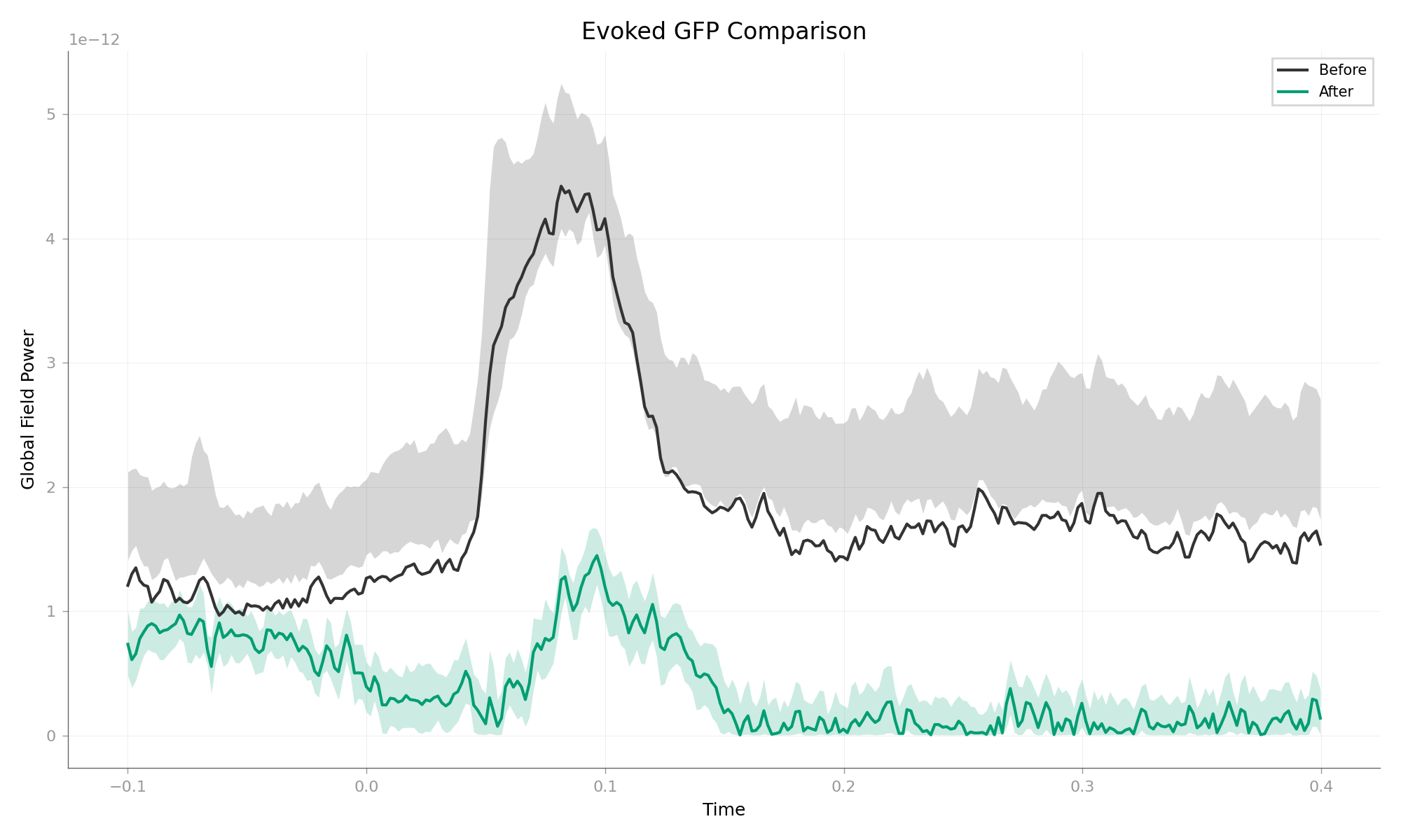
Evoked GFP Comparison
Reconstructing M100 component...
Not setting metadata
20 matching events found
No baseline correction applied
0 projection items activated

<Figure size 2000x1200 with 1 Axes>

Conclusion#

We successfully demonstrated the flexibility of DSS: AverageBias: Found phase-locked signals (Sine wave, M100) by averaging. BandpassBias: Found induced/oscillatory signals (50Hz, Alpha) by filtering.

The same algorithm, DSS, solved both problems simply by changing the definition of “interesting”.

Total running time of the script: (1 minutes 2.361 seconds)