Denoising Rhythms (Spectral DSS).

This example demonstrates how to use DSS to isolate oscillatory brain rhythms (e.g., Alpha, Beta) using spectral biases.

It covers bandpass-based extraction of a known frequency band, narrowband scanning to find oscillatory peaks automatically, and application to real MEG and EEG recordings.

Authors: Sina Esmaeili (sina.esmaeili@umontreal.ca)

Hamza Abdelhedi (hamza.abdelhedi@umontreal.ca)

Imports

import os

import matplotlib.pyplot as plt
import mne
import numpy as np
from mne.datasets import sample
from scipy import signal

from mne_denoise.dss import DSS, BandpassBias, LineNoiseBias
from mne_denoise.dss.variants import narrowband_dss, narrowband_scan
from mne_denoise.viz import (
    plot_component_psd_comparison,
    plot_component_summary,
    plot_narrowband_score_scan,
)

Part 0: Synthetic Data Demo

We simulate a brain-like mixture with an alpha rhythm at 10 Hz in one set of channels, a beta rhythm at 22 Hz in another set, plus pink noise and a 60 Hz line component.

print("\n--- Part 0: Synthetic Data Demo ---")

rng = np.random.default_rng(42)
sfreq = 500
n_seconds = 20
n_times = n_seconds * sfreq
n_channels = 16
times = np.arange(n_times) / sfreq

# 1. Generate Noise (Pink + Line)
noise = np.cumsum(rng.standard_normal((n_channels, n_times)), axis=1)  # Brownian/Pink
noise = signal.detrend(noise, axis=1)
noise += 0.5 * np.sin(2 * np.pi * 60 * times)  # Line noise

# 2. Generate Rhythms
# Alpha (10 Hz) - Amplitude Modulated
alpha_env = np.sin(2 * np.pi * 0.5 * times) ** 2
alpha = alpha_env * np.sin(2 * np.pi * 10 * times) * 2.0

# Beta (22 Hz) - Constant
beta = np.sin(2 * np.pi * 22 * times) * 1.5

# 3. Mix into data
data = noise.copy()
# Alpha in ch 0-2
data[0:3] += alpha * np.array([[1.0], [0.8], [0.5]])
# Beta in ch 4-6
data[4:7] += beta * np.array([[1.0], [0.8], [0.5]])

print(f"Simulated {n_channels} ch x {n_seconds} s. Peaks at 10Hz and 22Hz.")

# Create MNE Raw with channel names and montage for topomap plotting
ch_names = [
    "Oz",
    "O1",
    "O2",
    "Pz",
    "P3",
    "P4",
    "P7",
    "P8",
    "Cz",
    "C3",
    "C4",
    "Fz",
    "F3",
    "F4",
    "F7",
    "F8",
]
info_sim = mne.create_info(ch_names, sfreq, "eeg")
montage = mne.channels.make_standard_montage("standard_1020")
info_sim.set_montage(montage)
raw_sim = mne.io.RawArray(data, info_sim)

--- Part 0: Synthetic Data Demo ---
Simulated 16 ch x 20 s. Peaks at 10Hz and 22Hz.
Creating RawArray with float64 data, n_channels=16, n_times=10000
    Range : 0 ... 9999 =      0.000 ...    19.998 secs
Ready.

Part 1: Narrowband Scan

Suppose we don’t know the frequencies. We can scan for them. narrowband_scan runs DSS at many frequencies and returns the “score” (eigenvalue).

print("\nScanning frequencies (5-30 Hz)...")
# We scan 5-30 Hz with 1 Hz resolution
# For each freq, it tries to find a component that is 'narrowband' at that freq.
best_dss, freqs, eigenvalues = narrowband_scan(
    data, sfreq=sfreq, freq_range=(5, 30), freq_step=0.5, bandwidth=2.0, n_components=1
)

# Visualize the Spectrum of "Oscillatoriness"
plot_narrowband_score_scan(freqs, eigenvalues, true_freqs=[10, 22], show=False)
plt.show()

print("Peaks clearly visible at 10 Hz and 22 Hz.")

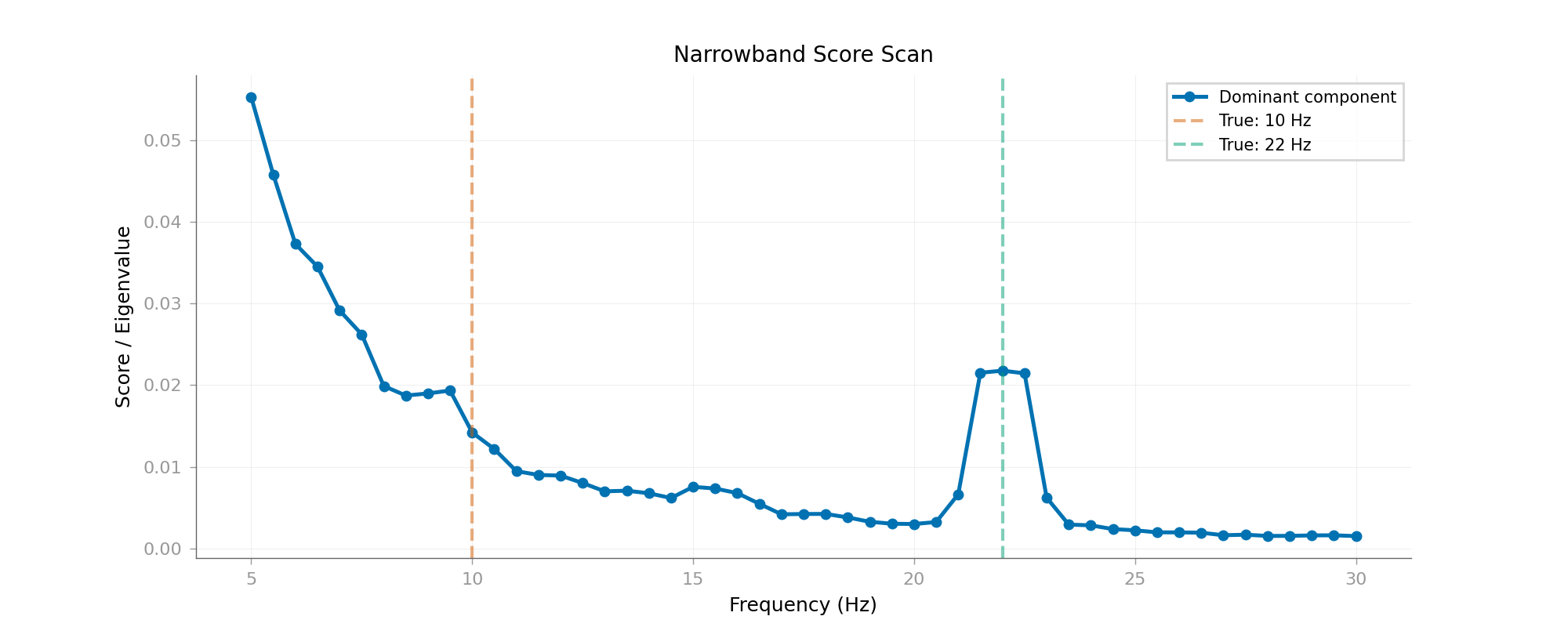
Scanning frequencies (5-30 Hz)...
Peaks clearly visible at 10 Hz and 22 Hz.

Part 1: Manual BandpassBias (10 Hz Alpha)

BandpassBias applies a bandpass filter as the bias function. Here we manually create it to understand the API.

print("\n--- Part 1a: Manual BandpassBias ---")

# Create BandpassBias for 10 Hz ± 1 Hz
bias_alpha = BandpassBias(freq_band=(9.0, 11.0), sfreq=sfreq, order=4)

# Fit DSS manually
dss_manual = DSS(n_components=4, bias=bias_alpha)
dss_manual.fit(raw_sim)

print(f"DSS Eigenvalues: {dss_manual.eigenvalues_[:4]}")

# Visualize
sources_manual = dss_manual.transform(raw_sim)
plot_component_summary(
    dss_manual,
    data=raw_sim,
    info=raw_sim.info,
    picks=np.arange(len(raw_sim.ch_names)),
    n_components=3,
    show=False,
)
plt.gcf().suptitle("Manual BandpassBias (9-11 Hz)")
plt.show()

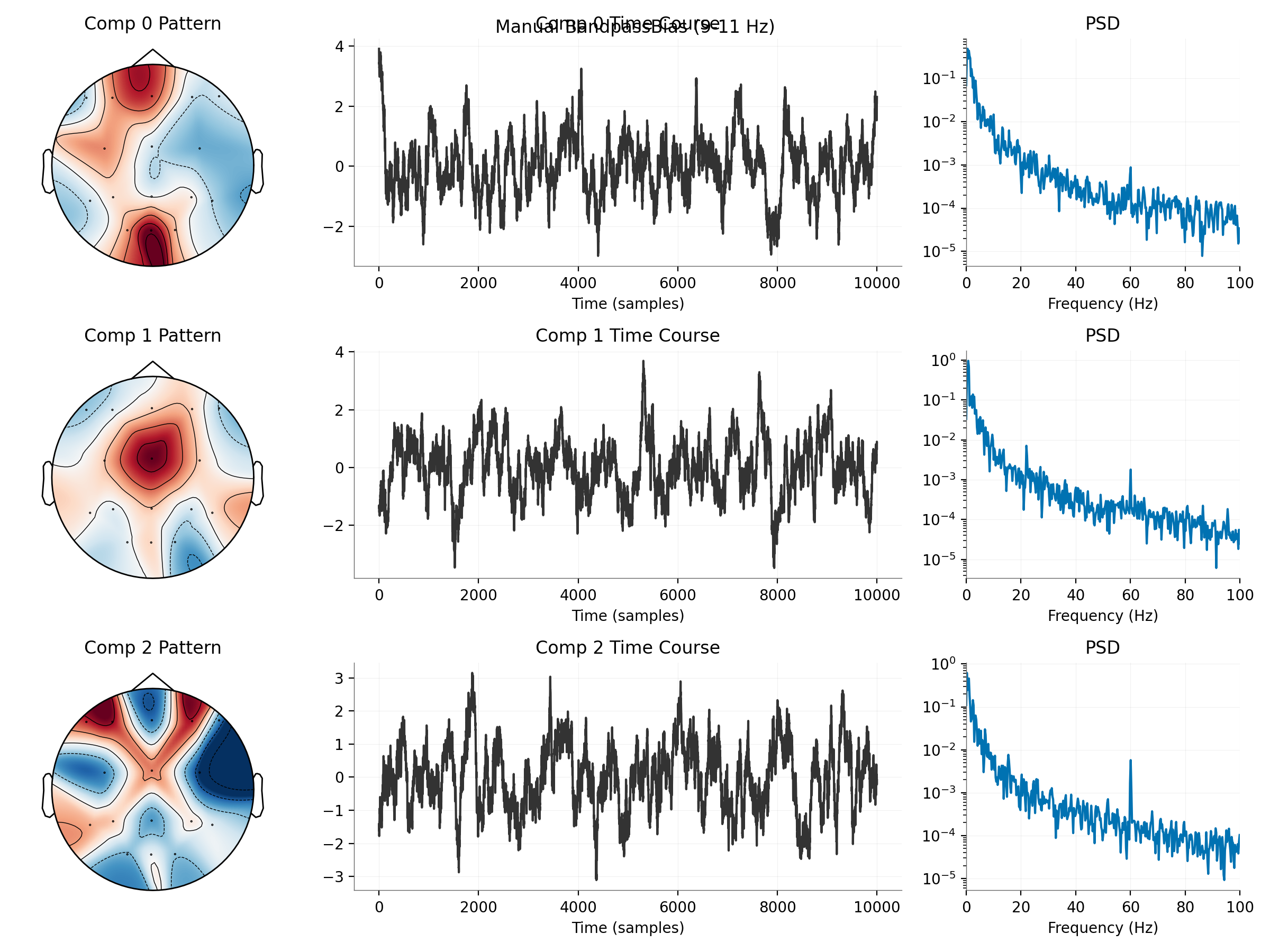
--- Part 1a: Manual BandpassBias ---
DSS Eigenvalues: [0.01420774 0.01187395 0.00853639 0.00608775]

Part 1b: Narrowband DSS Wrapper (Convenience)

The narrowband_dss() wrapper simplifies the above by calculating the frequency band automatically from center freq + bandwidth.

print("\n--- Part 1b: narrowband_dss Wrapper ---")

dss_alpha = narrowband_dss(sfreq=sfreq, freq=10.0, bandwidth=2.0, n_components=4)
dss_alpha.fit(raw_sim)

print(f"Wrapper DSS Eigenvalues: {dss_alpha.eigenvalues_[:4]}")
print("(Should be similar to manual approach)")

# Visualize extracted component PSD
sources = dss_alpha.transform(raw_sim)
comp_raw = mne.io.RawArray(sources, mne.create_info(4, sfreq, "eeg"))

fig = comp_raw.compute_psd(fmax=40).plot(show=False)
fig.suptitle("DSS Component Spectrum (Target: 10 Hz)")
plt.show()

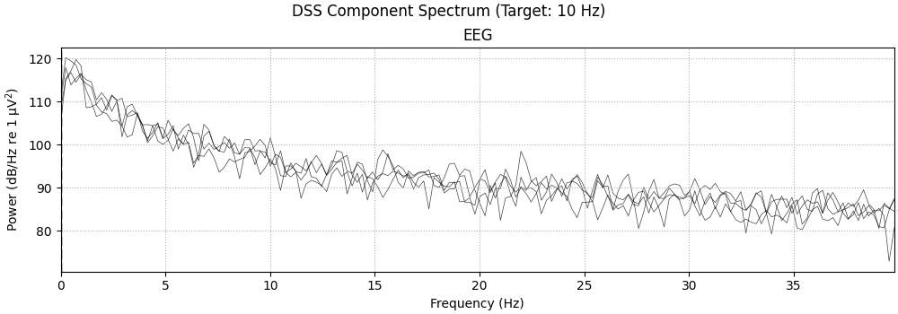
--- Part 1b: narrowband_dss Wrapper ---
Wrapper DSS Eigenvalues: [0.01420774 0.01187395 0.00853639 0.00608775]
(Should be similar to manual approach)
Creating RawArray with float64 data, n_channels=4, n_times=10000
    Range : 0 ... 9999 =      0.000 ...    19.998 secs
Ready.
Effective window size : 4.096 (s)
Plotting power spectral density (dB=True).
/home/runner/work/mne-denoise/mne-denoise/examples/dss/plot_04_spectral_dss.py:166: RuntimeWarning: Channel locations not available. Disabling spatial colors.
  fig = comp_raw.compute_psd(fmax=40).plot(show=False)

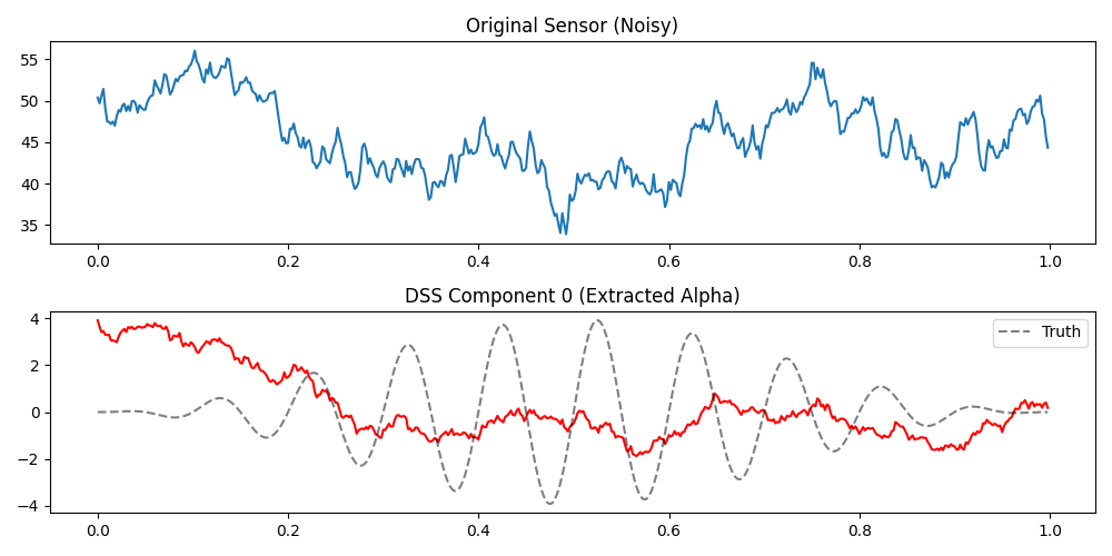
Compare Time Series

plt.figure(figsize=(10, 5))
plt.subplot(2, 1, 1)
plt.plot(times[:500], raw_sim.get_data()[0, :500])
plt.title("Original Sensor (Noisy)")
plt.subplot(2, 1, 2)
# Align polarity for visual comparison
src = sources[0, :500]
if np.corrcoef(src, alpha[:500])[0, 1] < 0:
    src *= -1
plt.plot(times[:500], src, "r")
plt.plot(
    times[:500],
    alpha[:500] * (np.max(np.abs(src)) / np.max(np.abs(alpha))),
    "k--",
    alpha=0.5,
    label="Truth",
)
plt.title("DSS Component 0 (Extracted Alpha)")
plt.legend()
plt.tight_layout()
plt.show()

Part 3: Line Noise Removal (LineNoiseBias)

LineNoiseBias isolates narrow frequency bands for removal (e.g., 60 Hz line noise). It supports both ‘iir’ (notch) and ‘fft’ (harmonic) methods.

print("\n--- Part 2: Line Noise (NotchBias) ---")

# Simulate data with 60 Hz line noise + harmonics
line_freq = 60.0  # Hz
line_noise = (
    0.5 * np.sin(2 * np.pi * line_freq * times)  # 60 Hz
    + 0.3 * np.sin(2 * np.pi * 2 * line_freq * times)  # 120 Hz
    + 0.1 * np.sin(2 * np.pi * 3 * line_freq * times)  # 180 Hz
)

# Add to alpha signal
data_noisy = data + np.outer(np.ones(n_channels), line_noise)
raw_noisy = mne.io.RawArray(data_noisy, info_sim)

print(f"Added {line_freq} Hz line noise + harmonics")

--- Part 2: Line Noise (NotchBias) ---
Creating RawArray with float64 data, n_channels=16, n_times=10000
    Range : 0 ... 9999 =      0.000 ...    19.998 secs
Ready.
Added 60.0 Hz line noise + harmonics

Apply DSS with LineNoiseBias to Remove 60 Hz

# We use method='iir' to replicate a traditional Notch filter approach
notch_bias_60 = LineNoiseBias(freq=60, sfreq=sfreq, method="iir", bandwidth=2)
dss_notch = DSS(n_components=None, bias=notch_bias_60)
dss_notch.fit(raw_noisy)

print(f"\nDSS Eigenvalues: {dss_notch.eigenvalues_[:3]}")
print("Component 0 should capture 60 Hz line noise")

sources_notch = dss_notch.transform(raw_noisy)

# Visualize
plot_component_summary(
    dss_notch,
    data=raw_noisy,
    info=raw_noisy.info,
    picks=np.arange(len(raw_noisy.ch_names)),
    n_components=3,
    show=False,
)
plt.show()

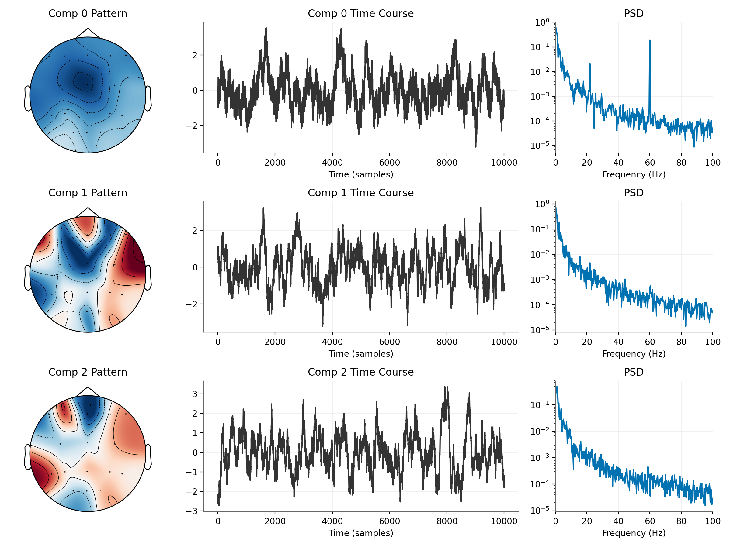
DSS Eigenvalues: [0.06828558 0.00038516 0.0002469 ]
Component 0 should capture 60 Hz line noise

PSD comparison

plot_component_psd_comparison(
    raw_noisy,
    sources_notch,
    component_indices=[0],
    sfreq=sfreq,
    peak_freq=60,
    fmax=200,
    show=False,
)
plt.gcf().axes[0].set_title("Line Noise: Original PSD (60 Hz + harmonics)")
plt.gcf().axes[1].set_title("Line Noise: DSS Components PSD")
# Mark harmonics
for ax in plt.gcf().axes:
    for h in [2, 3]:
        ax.axvline(line_freq * h, color="orange", linestyle="--", alpha=0.5)
plt.show()

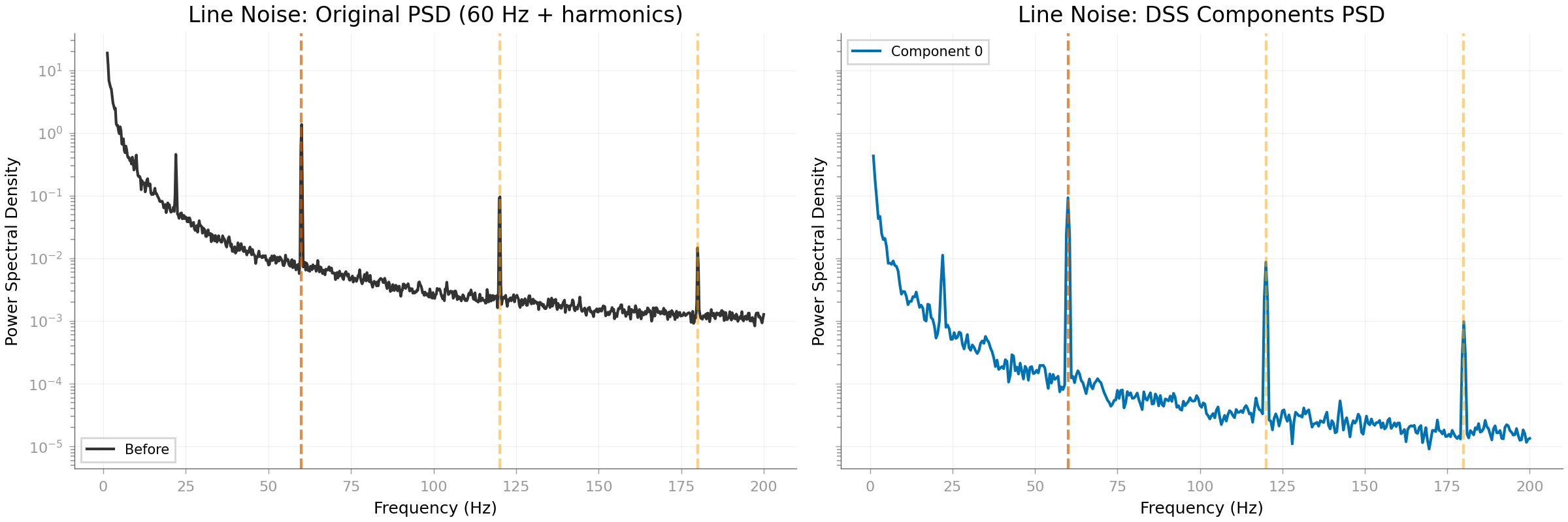
Effective window size : 4.096 (s)

Remove Line Noise and Recover Clean Signal

Project out the first component (60 Hz noise)

# Get denoised data by removing component 0
sources = dss_notch.transform(raw_noisy)
sources[0] = 0  # Zero out the 60 Hz component

# Reconstruct without line noise
data_cleaned = dss_notch.inverse_transform(sources)

# Compare PSDs
from scipy.signal import welch

freqs_orig, psd_orig = welch(data_noisy[0], fs=sfreq, nperseg=1024)
freqs_clean, psd_clean = welch(data_cleaned[0], fs=sfreq, nperseg=1024)

plt.figure(figsize=(10, 5))
plt.semilogy(freqs_orig, psd_orig, "r", alpha=0.7, label="With 60 Hz noise")
plt.semilogy(freqs_clean, psd_clean, "g", alpha=0.7, label="After removal")
plt.axvline(60, color="k", linestyle="--", alpha=0.5, label="60 Hz")
plt.axvline(120, color="gray", linestyle="--", alpha=0.5)
plt.xlabel("Frequency (Hz)")
plt.ylabel("Power")
plt.title("Line Noise Removal with LineNoiseBias")
plt.legend()
plt.xlim(0, 200)
plt.grid(True, alpha=0.3)
plt.show()

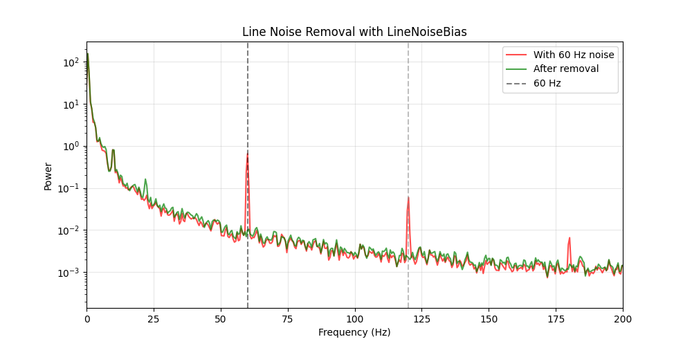
Part 4: Real Data (MEG Alpha)

We apply this to real MEG data to find spontaneous Alpha rhythms.

print("\n--- Part 3: MNE Sample Data (Alpha) ---")

home = os.path.expanduser("~")
mne_data_path = os.path.join(home, "mne_data")
data_path = sample.data_path()
raw_fname = data_path / "MEG" / "sample" / "sample_audvis_raw.fif"
raw = mne.io.read_raw_fif(raw_fname, preload=True, verbose=False)
raw.pick_types(meg="grad", eeg=False, eog=False, stim=False, exclude="bads")
raw.crop(0, 60)  # 60 seconds
raw.resample(100)  # Downsample for speed

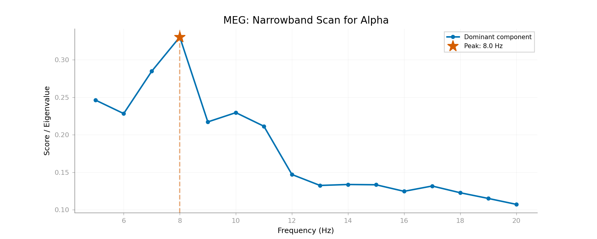
# Scan for natural rhythms in this dataset
print("Scanning MEG data 5-20 Hz...")
_, freqs_meg, eigs_meg = narrowband_scan(
    raw.get_data(),
    sfreq=raw.info["sfreq"],
    freq_range=(5, 20),
    freq_step=1.0,
    n_components=1,
)

plot_narrowband_score_scan(
    freqs_meg, eigs_meg, peak_freq=freqs_meg[np.argmax(eigs_meg)], show=False
)
plt.gcf().axes[0].set_title("MEG: Narrowband Scan for Alpha")
plt.show()

# Typically ~10-11 Hz is dominant. Let's extract it.
peak_freq = freqs_meg[np.argmax(eigs_meg)]
print(f"Peak detected at {peak_freq:.1f} Hz")

dss_meg = narrowband_dss(
    sfreq=raw.info["sfreq"], freq=peak_freq, bandwidth=3.0, n_components=5
)
dss_meg.fit(raw)

--- Part 3: MNE Sample Data (Alpha) ---
NOTE: pick_types() is a legacy function. New code should use inst.pick(...).
Scanning MEG data 5-20 Hz...
Peak detected at 8.0 Hz

DSS(bias=<mne_denoise.dss.denoisers.spectral.BandpassBias object at 0x7f64589bb6e0>,
    n_components=5)

In a Jupyter environment, please rerun this cell to show the HTML representation or trust the notebook.
On GitHub, the HTML representation is unable to render, please try loading this page with nbviewer.org.

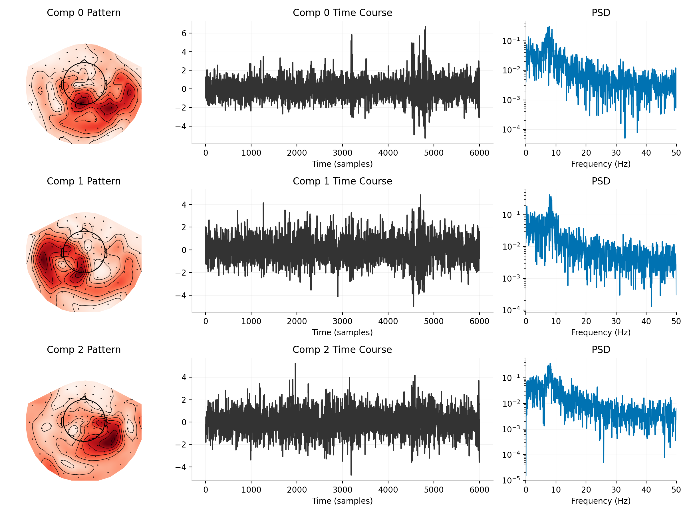
plot_component_summary(
    dss_meg,
    data=raw,
    info=raw.info,
    picks=np.arange(len(raw.ch_names)),
    n_components=3,
    show=False,
)
plt.show()

Additional visualizations for MEG

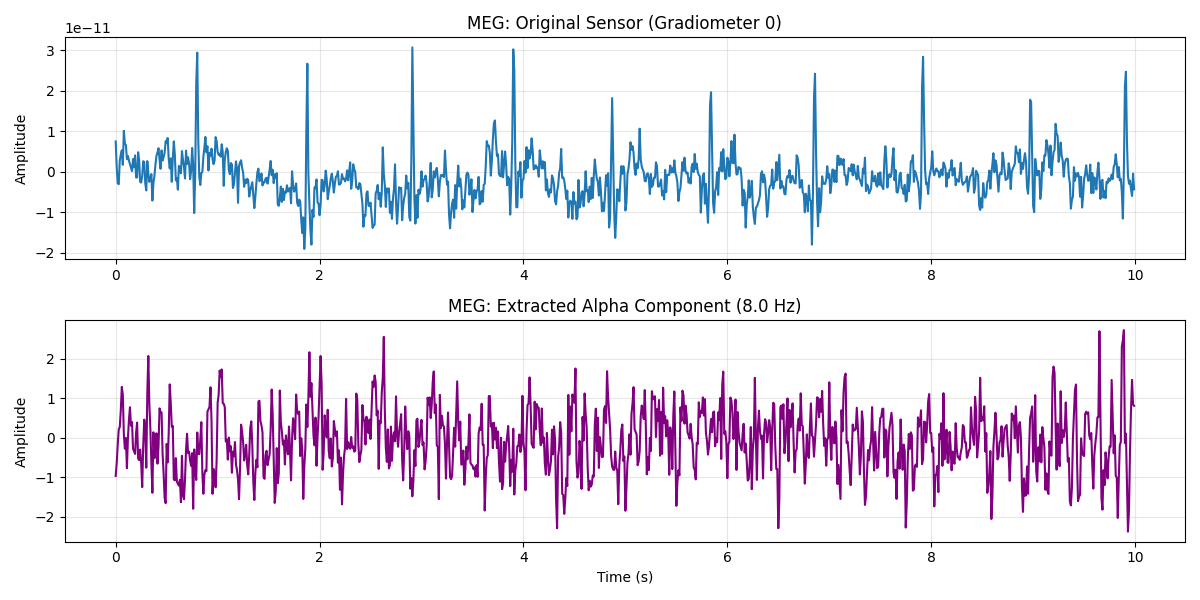
print("Creating additional MEG visualizations...")

# The high-level visualization helpers can also produce the same comparisons,
# but here we keep custom plots so the intermediate quantities remain explicit.

# Time series comparison: Raw sensor vs DSS component
sources_meg = dss_meg.transform(raw)
fig, axes = plt.subplots(2, 1, figsize=(12, 6))
t = raw.times[:1000]  # First 10 seconds
axes[0].plot(t, raw.get_data()[0, :1000])
axes[0].set_title("MEG: Original Sensor (Gradiometer 0)")
axes[0].set_ylabel("Amplitude")
axes[0].grid(True, alpha=0.3)
axes[1].plot(t, sources_meg[0, :1000], color="purple")
axes[1].set_title(f"MEG: Extracted Alpha Component ({peak_freq:.1f} Hz)")
axes[1].set_xlabel("Time (s)")
axes[1].set_ylabel("Amplitude")
axes[1].grid(True, alpha=0.3)
plt.tight_layout()
plt.show()

Creating additional MEG visualizations...

PSD Comparison: Before vs After

plot_component_psd_comparison(
    raw,
    sources_meg,
    component_indices=[0],
    sfreq=raw.info["sfreq"],
    peak_freq=peak_freq,
    show=False,
)
plt.gcf().axes[0].set_title("MEG: Original Data PSD (Average)")
plt.gcf().axes[1].set_title("MEG: DSS Components PSD")
plt.show()

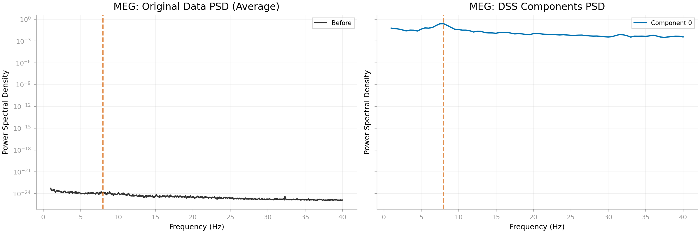
Effective window size : 20.480 (s)

Part 4: Real Data (EEG Alpha - Resting State)

For EEG, we use the EEG Motor Movement/Imagery dataset which includes resting-state recordings with eyes-open and eyes-closed conditions. Eyes-closed resting state typically shows strong alpha rhythms (8-12 Hz).

print("\n--- Part 4: EEG Resting-State Alpha (EEGBCI Dataset) ---")

from mne.datasets import eegbci
from mne.io import read_raw_edf

# Load resting-state data (eyes closed = run 1)
# Subject 1, Run 1 (eyes closed 1 minute)
print("Loading EEGBCI resting-state data (eyes closed)...")
raw_eeg = read_raw_edf(
    eegbci.load_data(subjects=[1], runs=[1], update_path=True)[0],
    preload=True,
    verbose=False,
)

# Clean up annotations
raw_eeg.annotations.onset[:] = 0  # Reset annotations
eegbci.standardize(raw_eeg)  # Apply standard channel names
montage = mne.channels.make_standard_montage("standard_1005")
raw_eeg.set_montage(montage, on_missing="ignore")

# Pick EEG channels, exclude non-standard ones
raw_eeg.pick_types(meg=False, eeg=True, stim=False, eog=False, exclude="bads")
raw_eeg.crop(0, 30)  # Use first 30 seconds
raw_eeg.filter(1, 40, fir_design="firwin")  # Bandpass for cleaner alpha
raw_eeg.resample(100)  # Downsample for speed

# Re-reference to average
raw_eeg.set_eeg_reference("average", projection=True)
raw_eeg.apply_proj()

print(
    f"EEG Data: {len(raw_eeg.ch_names)} channels, "
    f"{raw_eeg.times[-1]:.1f}s (eyes closed)"
)

# Scan for rhythms
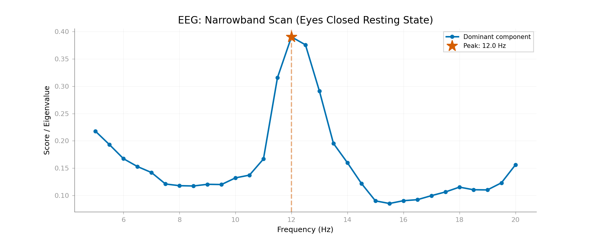
print("Scanning EEG for alpha rhythm...")
_, freqs_eeg, eigs_eeg = narrowband_scan(
    raw_eeg.get_data(),
    sfreq=raw_eeg.info["sfreq"],
    freq_range=(5, 20),
    freq_step=0.5,
    n_components=1,
)

peak_freq_eeg = freqs_eeg[np.argmax(eigs_eeg)]
plot_narrowband_score_scan(freqs_eeg, eigs_eeg, peak_freq=peak_freq_eeg, show=False)
plt.gcf().axes[0].set_title("EEG: Narrowband Scan (Eyes Closed Resting State)")
plt.show()

print(f"EEG Peak detected at {peak_freq_eeg:.1f} Hz (alpha band)")

# Extract alpha component
dss_eeg = narrowband_dss(
    sfreq=raw_eeg.info["sfreq"], freq=peak_freq_eeg, bandwidth=3.0, n_components=5
)
dss_eeg.fit(raw_eeg)

--- Part 4: EEG Resting-State Alpha (EEGBCI Dataset) ---
Loading EEGBCI resting-state data (eyes closed)...
Using default location ~/mne_data for EEGBCI...
Downloading EEGBCI data
Download complete in 08s (1.2 MB)
NOTE: pick_types() is a legacy function. New code should use inst.pick(...).
Filtering raw data in 1 contiguous segment
Setting up band-pass filter from 1 - 40 Hz

FIR filter parameters
---------------------
Designing a one-pass, zero-phase, non-causal bandpass filter:
- Windowed time-domain design (firwin) method
- Hamming window with 0.0194 passband ripple and 53 dB stopband attenuation
- Lower passband edge: 1.00
- Lower transition bandwidth: 1.00 Hz (-6 dB cutoff frequency: 0.50 Hz)
- Upper passband edge: 40.00 Hz
- Upper transition bandwidth: 10.00 Hz (-6 dB cutoff frequency: 45.00 Hz)
- Filter length: 529 samples (3.306 s)

EEG channel type selected for re-referencing
Adding average EEG reference projection.
1 projection items deactivated
Average reference projection was added, but has not been applied yet. Use the apply_proj method to apply it.
Created an SSP operator (subspace dimension = 1)
1 projection items activated
SSP projectors applied...
EEG Data: 64 channels, 30.0s (eyes closed)
Scanning EEG for alpha rhythm...
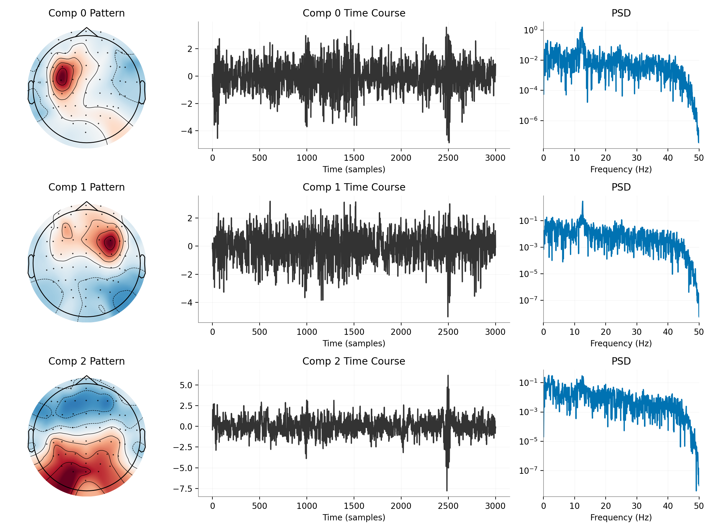
EEG Peak detected at 12.0 Hz (alpha band)

DSS(bias=<mne_denoise.dss.denoisers.spectral.BandpassBias object at 0x7f6459338230>,
    n_components=5)

In a Jupyter environment, please rerun this cell to show the HTML representation or trust the notebook.
On GitHub, the HTML representation is unable to render, please try loading this page with nbviewer.org.

plot_component_summary(
    dss_eeg,
    data=raw_eeg,
    info=raw_eeg.info,
    picks=np.arange(len(raw_eeg.ch_names)),
    n_components=3,
    show=False,
)
plt.show()

Additional visualizations for EEG

print("Creating additional EEG visualizations...")

# Note: Similar to MEG, you can use plot_psd_comparison() and
# plot_channel_time_course_comparison() from mne_denoise.viz

# Time series comparison: Raw sensor vs DSS component
sources_eeg = dss_eeg.transform(raw_eeg)
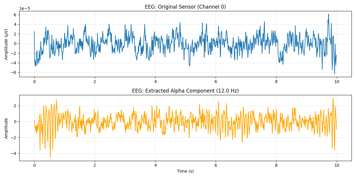
fig, axes = plt.subplots(2, 1, figsize=(12, 6))
t_eeg = raw_eeg.times[:1000]  # First 10 seconds
axes[0].plot(t_eeg, raw_eeg.get_data()[0, :1000])
axes[0].set_title("EEG: Original Sensor (Channel 0)")
axes[0].set_ylabel("Amplitude (µV)")
axes[0].grid(True, alpha=0.3)
axes[1].plot(t_eeg, sources_eeg[0, :1000], color="orange")
axes[1].set_title(f"EEG: Extracted Alpha Component ({peak_freq_eeg:.1f} Hz)")
axes[1].set_xlabel("Time (s)")
axes[1].set_ylabel("Amplitude")
axes[1].grid(True, alpha=0.3)
plt.tight_layout()
plt.show()

Creating additional EEG visualizations...

PSD Comparison: Before vs After

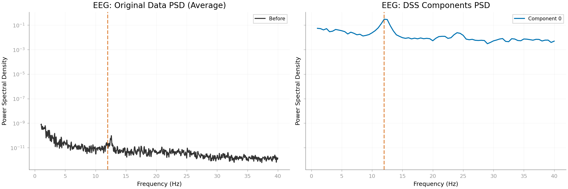
plot_component_psd_comparison(
    raw_eeg,
    sources_eeg,
    component_indices=[0],
    sfreq=raw_eeg.info["sfreq"],
    peak_freq=peak_freq_eeg,
    show=False,
)
plt.gcf().axes[0].set_title("EEG: Original Data PSD (Average)")
plt.gcf().axes[1].set_title("EEG: DSS Components PSD")
plt.show()

Effective window size : 20.480 (s)