Note
Go to the end to download the full example code.
Kernel OPM phantom data#
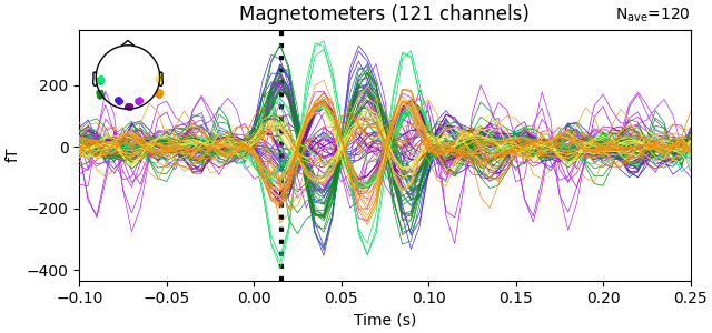
In this dataset, a Neuromag phantom was placed inside the Kernel OPM helmet and stimulated with 7 modules active (121 channels). Here we show some example traces.
# Authors: The MNE-Python contributors.
# License: BSD-3-Clause
# Copyright the MNE-Python contributors.

import numpy as np

import mne

data_path = mne.datasets.phantom_kernel.data_path()
fname = data_path / "phantom_32_100nam_raw.fif"
raw = mne.io.read_raw_fif(fname).load_data()
events = mne.find_events(raw, stim_channel="STI101")

# Bads identified by inspecting averages
raw.info["bads"] = [
    "RC2.bx.ave",
    "LC3.bx.ave",
    "RC2.by.7",
    "RC2.bz.7",
    "RC2.bx.4",
    "RC2.by.4",
    "LC3.bx.5",
]
# Drop the module-average channels
raw.drop_channels([ch_name for ch_name in raw.ch_names if ".ave" in ch_name])
# Add field correction projectors
raw.add_proj(mne.preprocessing.compute_proj_hfc(raw.info, order=2))
raw.pick("meg", exclude="bads")
raw.filter(0.5, 40)
epochs = mne.Epochs(
    raw,
    events,
    tmin=-0.1,
    tmax=0.25,
    decim=5,
    preload=True,
    baseline=(None, 0),
)
evoked = epochs["17"].average()  # a high-SNR dipole for these data
fig = evoked.plot()
t_peak = 0.016  # based on visual inspection of evoked
fig.axes[0].axvline(t_peak, color="k", ls=":", lw=3, zorder=2)
Opening raw data file /home/circleci/mne_data/MNE-phantom-kernel-data/phantom_32_100nam_raw.fif...
    Range : 0 ... 526631 =      0.000 ...   526.631 secs
Ready.
Reading 0 ... 526631  =      0.000 ...   526.631 secs...
Finding events on: STI101
1903 events found on stim channel STI101
Event IDs: [ 1  2  3  4  5  6  7  8  9 10 11 12 13 14 15 16 17 18 19 20 21 22 23 24
 25 26 27 28 29 30 31 32]
8 projection items deactivated
Filtering raw data in 1 contiguous segment
Setting up band-pass filter from 0.5 - 40 Hz

FIR filter parameters
---------------------
Designing a one-pass, zero-phase, non-causal bandpass filter:
- Windowed time-domain design (firwin) method
- Hamming window with 0.0194 passband ripple and 53 dB stopband attenuation
- Lower passband edge: 0.50
- Lower transition bandwidth: 0.50 Hz (-6 dB cutoff frequency: 0.25 Hz)
- Upper passband edge: 40.00 Hz
- Upper transition bandwidth: 10.00 Hz (-6 dB cutoff frequency: 45.00 Hz)
- Filter length: 6601 samples (6.601 s)

Not setting metadata
1903 matching events found
Setting baseline interval to [-0.1, 0.0] s
Applying baseline correction (mode: mean)
Created an SSP operator (subspace dimension = 8)
8 projection items activated
Using data from preloaded Raw for 1903 events and 351 original time points (prior to decimation) ...
0 bad epochs dropped
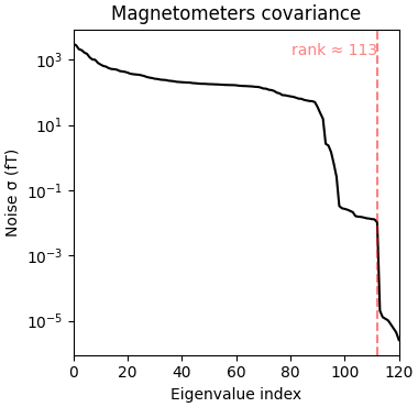
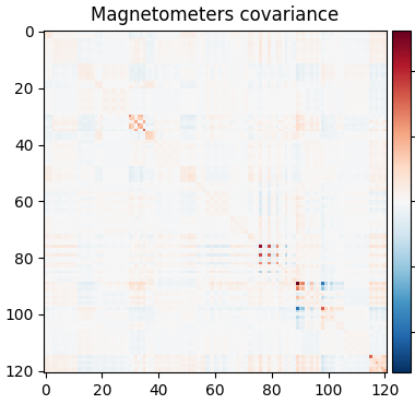
The data covariance has an interesting structure because of densely packed sensors:
cov = mne.compute_covariance(epochs, tmax=-0.01)
mne.viz.plot_cov(cov, raw.info)
    Created an SSP operator (subspace dimension = 8)
    Setting small MAG eigenvalues to zero (without PCA)
Reducing data rank from 121 -> 113
Estimating covariance using EMPIRICAL
Done.
Number of samples used : 36157
[done]
Computing rank from covariance with rank=None
    Using tolerance 2.5e-13 (2.2e-16 eps * 121 dim * 9.2  max singular value)
    Estimated rank (mag): 113
    MAG: rank 113 computed from 121 data channels with 0 projectors
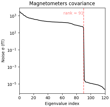
So let’s be careful and compute rank ahead of time and regularize:
rank = mne.compute_rank(epochs, tol=1e-3, tol_kind="relative")
cov = mne.compute_covariance(epochs, tmax=-0.01, rank=rank, method="shrunk")
mne.viz.plot_cov(cov, raw.info)
Computing rank from data with rank=None
    Estimated rank (mag): 91
    MAG: rank 91 computed from 121 data channels with 8 projectors
    Created an SSP operator (subspace dimension = 8)
    Setting small MAG eigenvalues to zero (without PCA)
Reducing data rank from 121 -> 91
Estimating covariance using SHRUNK
Done.
Number of samples used : 36157
[done]
Computing rank from covariance with rank=None
    Using tolerance 2.5e-13 (2.2e-16 eps * 121 dim * 9.2  max singular value)
    Estimated rank (mag): 91
    MAG: rank 91 computed from 121 data channels with 0 projectors
Look at our alignment:
sphere = mne.make_sphere_model(r0=(0.0, 0.0, 0.0), head_radius=0.08)
trans = mne.transforms.Transform("head", "mri", np.eye(4))
align_kwargs = dict(
    trans=trans,
    bem=sphere,
    surfaces={"outer_skin": 0.2},
    show_axes=True,
)
mne.viz.plot_alignment(
    raw.info,
    coord_frame="meg",
    meg=dict(sensors=1.0, helmet=0.05),
    **align_kwargs,
)
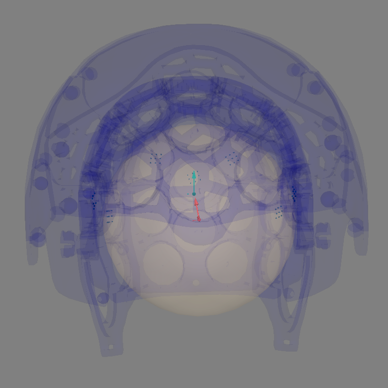
Equiv. model fitting -> RV = 0.00385873 %%
mu1 = 0.943736    lambda1 = 0.139585
mu2 = 0.66496    lambda2 = 0.685424
mu3 = -0.0416425    lambda3 = -0.0146395
Set up EEG sphere model with scalp radius    80.0 mm

Getting helmet for system Kernel_Flux
    Deforming CAD helmet to match 7 acquisition sensor positions:
    1. Affine: 4.8°, 4.6 mm, 1.00× scale
    2. Nonlinear displacement: mean=1.9, max=6.9 mm
Channel types:: mag: 121
Let’s do dipole fits, which are not great because the dev_head_t is approximate and the sensor coverage is sparse:
data = list()
for ii in range(1, 33):
    evoked = epochs[str(ii)][1:-1].average().crop(t_peak, t_peak)
    data.append(evoked.data[:, 0])
evoked = mne.EvokedArray(np.array(data).T, evoked.info, tmin=0.0)
del epochs
dip, residual = mne.fit_dipole(evoked, cov, sphere, n_jobs=None)
actual_pos, actual_ori = mne.dipole.get_phantom_dipoles()
actual_amp = np.ones(len(dip))  # fake amp, needed to create Dipole instance
actual_gof = np.ones(len(dip))  # fake GOF, needed to create Dipole instance
dip_true = mne.Dipole(dip.times, actual_pos, actual_amp, actual_ori, actual_gof)

fig = mne.viz.plot_alignment(
    evoked.info, coord_frame="head", meg="sensors", **align_kwargs
)
mne.viz.plot_dipole_locations(
    dipoles=dip_true, mode="arrow", color=(0.0, 0.0, 0.0), fig=fig
)
mne.viz.plot_dipole_locations(dipoles=dip, mode="arrow", color=(0.2, 1.0, 0.5), fig=fig)
mne.viz.set_3d_view(figure=fig, azimuth=30, elevation=70, distance=0.4)
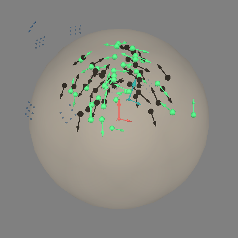
BEM               : <ConductorModel | Sphere (3 layers): r0=[0.0, 0.0, 0.0] R=80 mm>
MRI transform     : identity
Sphere model      : origin at (   0.00    0.00    0.00) mm, rad =    0.1 mm
Guess grid        :   20.0 mm
Guess mindist     :    5.0 mm
Guess exclude     :   20.0 mm
Using normal MEG coil definitions.
Noise covariance  : <Covariance | kind : full, shape : (121, 121), range : [-1.9e-24, +2.6e-24], n_samples : 36156>

Coordinate transformation: MRI (surface RAS) -> head
    1.000000 0.000000 0.000000       0.00 mm
    0.000000 1.000000 0.000000       0.00 mm
    0.000000 0.000000 1.000000       0.00 mm
    0.000000 0.000000 0.000000       1.00
Coordinate transformation: MEG device -> head
    0.981060 -0.039414 -0.189651       0.00 mm
    0.085832 0.966167 0.243215      10.00 mm
    0.173648 -0.254887 0.951251      20.00 mm
    0.000000 0.000000 0.000000       1.00
0 bad channels total
Read 121 MEG channels from info
105 coil definitions read
Coordinate transformation: MEG device -> head
    0.981060 -0.039414 -0.189651       0.00 mm
    0.085832 0.966167 0.243215      10.00 mm
    0.173648 -0.254887 0.951251      20.00 mm
    0.000000 0.000000 0.000000       1.00
MEG coil definitions created in head coordinates.
Decomposing the sensor noise covariance matrix...
    Created an SSP operator (subspace dimension = 8)
Computing rank from covariance with rank=None
    Using tolerance 2.5e-13 (2.2e-16 eps * 121 dim * 9.2  max singular value)
    Estimated rank (mag): 91
    MAG: rank 91 computed from 121 data channels with 8 projectors
    Setting small MAG eigenvalues to zero (without PCA)
    Created the whitener using a noise covariance matrix with rank 91 (30 small eigenvalues omitted)

---- Computing the forward solution for the guesses...
Making a spherical guess space with radius    72.0 mm...
Filtering (grid =     20 mm)...
Surface CM = (   0.0    0.0    0.0) mm
Surface fits inside a sphere with radius   72.0 mm
Surface extent:
    x =  -72.0 ...   72.0 mm
    y =  -72.0 ...   72.0 mm
    z =  -72.0 ...   72.0 mm
Grid extent:
    x =  -80.0 ...   80.0 mm
    y =  -80.0 ...   80.0 mm
    z =  -80.0 ...   80.0 mm
729 sources before omitting any.
178 sources after omitting infeasible sources not within 20.0 - 72.0 mm.
Source spaces are in MRI coordinates.
Checking that the sources are inside the surface and at least    5.0 mm away (will take a few...)
    8 source space point omitted because of the    5.0-mm distance limit.
170 sources remaining after excluding the sources outside the surface and less than    5.0 mm inside.
Go through all guess source locations...
[done 170 sources]
---- Fitted :     0.0 ms
---- Fitted :     5.0 ms
---- Fitted :    10.0 ms
---- Fitted :    15.0 ms
---- Fitted :    20.0 ms
---- Fitted :    25.0 ms
---- Fitted :    30.0 ms
---- Fitted :    35.0 ms
---- Fitted :    40.0 ms
---- Fitted :    45.0 ms
---- Fitted :    50.0 ms
---- Fitted :    55.0 ms
---- Fitted :    60.0 ms
---- Fitted :    65.0 ms
---- Fitted :    70.0 ms
---- Fitted :    75.0 ms
---- Fitted :    80.0 ms
---- Fitted :    85.0 ms
---- Fitted :    90.0 ms
---- Fitted :    95.0 ms
---- Fitted :   100.0 ms
---- Fitted :   105.0 ms
---- Fitted :   110.0 ms
---- Fitted :   115.0 ms
---- Fitted :   120.0 ms
---- Fitted :   125.0 ms
---- Fitted :   130.0 ms
---- Fitted :   135.0 ms
---- Fitted :   140.0 ms
---- Fitted :   145.0 ms
---- Fitted :   150.0 ms
---- Fitted :   155.0 ms
Projections have already been applied. Setting proj attribute to True.
32 time points fitted
Channel types:: mag: 121
Total running time of the script: (0 minutes 39.696 seconds)

