mne.Covariance#
- class mne.Covariance(data, names, bads, projs, nfree, eig=None, eigvec=None, method=None, loglik=None, *, verbose=None)[source]#
Noise covariance matrix.
Note
This class should not be instantiated directly via
mne.Covariance(...). Instead, use one of the functions listed in the See Also section below.- Parameters:
- dataarray_like
The data.
- names
listofstr Channel names.
- bads
listofstr Bad channels.
- projs
list Projection vectors.
- nfree
int Degrees of freedom.
- eigarray_like |
None Eigenvalues.
- eigvecarray_like |
None Eigenvectors.
- method
str|None The method used to compute the covariance.
- loglik
float The log likelihood.
- verbosebool |
str|int|None Control verbosity of the logging output. If
None, use the default verbosity level. See the logging documentation andmne.verbose()for details. Should only be passed as a keyword argument.
- Attributes:
Methods
__add__(cov)Add Covariance taking into account number of degrees of freedom.
__contains__(key, /)True if the dictionary has the specified key, else False.
__getitem__(key, /)Return self[key].
__iter__(/)Implement iter(self).
__len__(/)Return len(self).
as_diag()Set covariance to be processed as being diagonal.
clear()copy()Copy the Covariance object.
fromkeys(iterable[, value])Create a new dictionary with keys from iterable and values set to value.
get(key[, default])Return the value for key if key is in the dictionary, else default.
items()keys()pick_channels(ch_names[, ordered, verbose])Pick channels from this covariance matrix.
plot(info[, exclude, colorbar, proj, ...])Plot Covariance data.
plot_topomap(info[, ch_type, scalings, ...])Plot a topomap of the covariance diagonal.
pop(key[, default])If the key is not found, return the default if given; otherwise, raise a KeyError.
popitem(/)Remove and return a (key, value) pair as a 2-tuple.
save(fname, *[, overwrite, verbose])Save covariance matrix in a FIF file.
setdefault(key[, default])Insert key with a value of default if key is not in the dictionary.
update([E, ]**F)If E is present and has a .keys() method, then does: for k in E: D[k] = E[k] If E is present and lacks a .keys() method, then does: for k, v in E: D[k] = v In either case, this is followed by: for k in F: D[k] = F[k]
values()- __contains__(key, /)#
True if the dictionary has the specified key, else False.
- __getitem__(key, /)#
Return self[key].
- __iter__(/)#
Implement iter(self).
- __len__(/)#
Return len(self).
- as_diag()[source]#
Set covariance to be processed as being diagonal.
- Returns:
- cov
dict The covariance.
- cov
Notes
This function allows creation of inverse operators equivalent to using the old “–diagnoise” mne option.
This function operates in place.
- property ch_names#
Channel names.
- clear() None. Remove all items from D.#
- copy()[source]#
Copy the Covariance object.
- Returns:
- covinstance of
Covariance The copied object.
- covinstance of
Examples using
copy: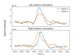
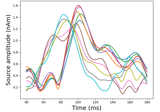
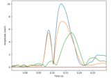
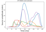
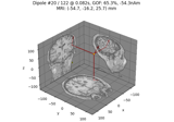
Computing source timecourses with an XFit-like multi-dipole model
Computing source timecourses with an XFit-like multi-dipole model
- property data#
Numpy array of Noise covariance matrix.
- classmethod fromkeys(iterable, value=None, /)#
Create a new dictionary with keys from iterable and values set to value.
- get(key, default=None, /)#
Return the value for key if key is in the dictionary, else default.
- items() a set-like object providing a view on D's items#
- keys() a set-like object providing a view on D's keys#
- property nfree#
Number of degrees of freedom.
- pick_channels(ch_names, ordered=True, *, verbose=None)[source]#
Pick channels from this covariance matrix.
- Parameters:
- ch_names
listofstr List of channels to keep. All other channels are dropped.
- orderedbool
If True (default), ensure that the order of the channels in the modified instance matches the order of
ch_names.New in v0.20.0.
Changed in version 1.7: The default changed from False in 1.6 to True in 1.7.
- verbosebool |
str|int|None Control verbosity of the logging output. If
None, use the default verbosity level. See the logging documentation andmne.verbose()for details. Should only be passed as a keyword argument.
- ch_names
- Returns:
- covinstance of Covariance.
The modified covariance matrix.
Notes
Operates in-place.
New in v0.20.0.
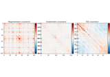
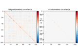
- plot(info, exclude=(), colorbar=True, proj=False, show_svd=True, show=True, verbose=None)[source]#
Plot Covariance data.
- Parameters:
- info
mne.Info The
mne.Infoobject with information about the sensors and methods of measurement.- exclude
listofstr|str List of channels to exclude. If empty do not exclude any channel. If ‘bads’, exclude info[‘bads’].
- colorbarbool
Show colorbar or not.
- projbool
Apply projections or not.
- show_svdbool
Plot also singular values of the noise covariance for each sensor type. We show square roots ie. standard deviations.
- showbool
Show figure if True.
- verbosebool |
str|int|None Control verbosity of the logging output. If
None, use the default verbosity level. See the logging documentation andmne.verbose()for details. Should only be passed as a keyword argument.
- info
- Returns:
- fig_covinstance of
matplotlib.figure.Figure The covariance plot.
- fig_svdinstance of
matplotlib.figure.Figure|None The SVD plot of the covariance (i.e., the eigenvalues or “matrix spectrum”).
- fig_covinstance of
See also
Notes
For each channel type, the rank is estimated using
mne.compute_rank().Changed in version 0.19: Approximate ranks for each channel type are shown with red dashed lines.
Examples using
plot: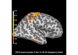
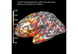
Compute evoked ERS source power using DICS, LCMV beamformer, and dSPM
Compute evoked ERS source power using DICS, LCMV beamformer, and dSPM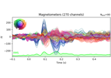
Working with CTF data: the Brainstorm auditory dataset
Working with CTF data: the Brainstorm auditory dataset
- plot_topomap(info, ch_type=None, *, scalings=None, proj=False, noise_cov=None, sensors=True, show_names=False, mask=None, mask_params=None, contours=6, outlines='head', sphere=None, image_interp='cubic', extrapolate='auto', border='mean', res=64, size=1, cmap=None, vlim=(None, None), cnorm=None, colorbar=True, cbar_fmt='%3.1f', units=None, axes=None, show=True, verbose=None)[source]#
Plot a topomap of the covariance diagonal.
- Parameters:
- info
mne.Info The
mne.Infoobject with information about the sensors and methods of measurement.- ch_type‘mag’ | ‘grad’ | ‘planar1’ | ‘planar2’ | ‘eeg’ |
None The channel type to plot. For
'grad', the gradiometers are collected in pairs and the RMS for each pair is plotted. IfNonethe first available channel type from order shown above is used. Defaults toNone.New in v0.21.
- scalings
dict|float|None The scalings of the channel types to be applied for plotting. If None, defaults to
dict(eeg=1e6, grad=1e13, mag=1e15).- projbool | ‘interactive’ | ‘reconstruct’
If true SSP projections are applied before display. If
'interactive', a check box for reversible selection of SSP projection vectors will be shown. If'reconstruct', projection vectors will be applied and then M/EEG data will be reconstructed via field mapping to reduce the signal bias caused by projection.Changed in version 0.21: Support for ‘reconstruct’ was added.
- noise_covinstance of
Covariance|None If not None, whiten the instance with
noise_covbefore plotting.- sensorsbool |
str Whether to add markers for sensor locations. If
str, should be a valid matplotlib format string (e.g.,'r+'for red plusses, see the Notes section ofplot()). IfTrue(the default), black circles will be used.- show_namesbool |
callable() If
True, show channel names next to each sensor marker. If callable, channel names will be formatted using the callable; e.g., to delete the prefix ‘MEG ‘ from all channel names, pass the functionlambda x: x.replace('MEG ', ''). Ifmaskis notNone, only non-masked sensor names will be shown.- mask
ndarrayof bool, shape (n_channels,) |None Array indicating channel(s) to highlight with a distinct plotting style. Array elements set to
Truewill be plotted with the parameters given inmask_params. Defaults toNone, equivalent to an array of allFalseelements.- mask_params
dict|None Additional plotting parameters for plotting significant sensors. Default (None) equals:
dict(marker='o', markerfacecolor='w', markeredgecolor='k',
        linewidth=0, markersize=4)
- contours
int| array_like The number of contour lines to draw. If
0, no contours will be drawn. If a positive integer, that number of contour levels are chosen using the matplotlib tick locator (may sometimes be inaccurate, use array for accuracy). If array-like, the array values are used as the contour levels. The values should be in µV for EEG, fT for magnetometers and fT/m for gradiometers. Ifcolorbar=True, the colorbar will have ticks corresponding to the contour levels. Default is6.- outlines‘head’ |
dict|None The outlines to be drawn. If ‘head’, the default head scheme will be drawn. If dict, each key refers to a tuple of x and y positions, the values in ‘mask_pos’ will serve as image mask. Alternatively, a matplotlib patch object can be passed for advanced masking options, either directly or as a function that returns patches (required for multi-axis plots). If None, nothing will be drawn. Defaults to ‘head’.
- sphere
float| array_like offloat| instance ofConductorModel|str|listofstr|None The sphere parameters to use for the head outline. Can be array-like of shape (4,) to give the X/Y/Z origin and radius in meters, or a single float to give just the radius (origin assumed 0, 0, 0). Can also be an instance of a spherical
ConductorModelto use the origin and radius from that object. Can also be astr, in which case:'auto': the sphere is fit to external digitization points first, and to external + EEG digitization points if the former fails.'eeglab': the head circle is defined by EEG electrodes'Fpz','Oz','T7', and'T8'(if'Fpz'is not present, it will be approximated from the coordinates of'Oz').'extra': the sphere is fit to external digitization points.'eeg': the sphere is fit to EEG digitization points.'cardinal': the sphere is fit to cardinal digitization points.'hpi': the sphere is fit to HPI coil digitization points.
Can also be a list of
str, in which case the sphere is fit to the specified digitization points, which can be any combination of'extra','eeg','cardinal', and'hpi', as specified above.None(the default) is equivalent to'auto'when enough extra digitization points are available, and (0, 0, 0, 0.095) otherwise.New in v0.20.
Changed in version 1.1: Added
'eeglab'option.Changed in version 1.11: Added
'extra','eeg','cardinal','hpi'and list ofstroptions.- image_interp
str The image interpolation to be used. Options are
'cubic'(default) to usescipy.interpolate.CloughTocher2DInterpolator,'nearest'to usescipy.spatial.Voronoior'linear'to usescipy.interpolate.LinearNDInterpolator.- extrapolate
str Options:
'box'Extrapolate to four points placed to form a square encompassing all data points, where each side of the square is three times the range of the data in the respective dimension.
'local'(default for MEG sensors)Extrapolate only to nearby points (approximately to points closer than median inter-electrode distance). This will also set the mask to be polygonal based on the convex hull of the sensors.
'head'(default for non-MEG sensors)Extrapolate out to the edges of the clipping circle. This will be on the head circle when the sensors are contained within the head circle, but it can extend beyond the head when sensors are plotted outside the head circle.
Changed in version 0.21:
The default was changed to
'local'for MEG sensors.'local'was changed to use a convex hull mask'head'was changed to extrapolate out to the clipping circle.
- border
float| ‘mean’ Value to extrapolate to on the topomap borders. If
'mean'(default), then each extrapolated point has the average value of its neighbours.New in v0.20.
- res
int The resolution of the topomap image (number of pixels along each side).
- size
float Side length of each subplot in inches.
- cmapmatplotlib colormap | (colormap, bool) | ‘interactive’ |
None Colormap to use. If
tuple, the first value indicates the colormap to use and the second value is a boolean defining interactivity. In interactive mode the colors are adjustable by clicking and dragging the colorbar with left and right mouse button. Left mouse button moves the scale up and down and right mouse button adjusts the range. Hitting space bar resets the range. Up and down arrows can be used to change the colormap. IfNone,'Reds'is used for data that is either all-positive or all-negative, and'RdBu_r'is used otherwise.'interactive'is equivalent to(None, True). Defaults toNone.Warning
Interactive mode works smoothly only for a small amount of topomaps. Interactive mode is disabled by default for more than 2 topomaps.
- vlim
tupleof length 2 Lower and upper bounds of the colormap, typically a numeric value in the same units as the data. If both entries are
None, the bounds are set at(min(data), max(data)). ProvidingNonefor just one entry will set the corresponding boundary at the min/max of the data. Defaults to(None, None).New in v1.2.
- cnorm
matplotlib.colors.Normalize|None How to normalize the colormap. If
None, standard linear normalization is performed. If notNone,vminandvmaxwill be ignored. See Matplotlib docs for more details on colormap normalization, and the ERDs example for an example of its use.New in v1.2.
- colorbarbool
Plot a colorbar in the rightmost column of the figure.
- cbar_fmt
str Formatting string for colorbar tick labels. See Format specification mini-language for details.
- units
dict|str|None The units to use for the colorbar label. Ignored if
colorbar=False. IfNoneandscalings=Nonethe unit is automatically determined, otherwise the label will be “AU” indicating arbitrary units. Default isNone.- axesinstance of
Axes|listofAxes|None The axes to plot into. If
None, a newFigurewill be created with the correct number of axes. IfAxesare provided (either as a single instance or alistof axes), the number of axes provided must be length 1. Default isNone.- showbool
Show the figure if
True.- verbosebool |
str|int|None Control verbosity of the logging output. If
None, use the default verbosity level. See the logging documentation andmne.verbose()for details. Should only be passed as a keyword argument.
- info
- Returns:
- figinstance of
Figure The matplotlib figure.
- figinstance of
Notes
New in v0.21.
Examples using
plot_topomap:
Compute source power estimate by projecting the covariance with MNE
Compute source power estimate by projecting the covariance with MNE
- pop(key, default=<unrepresentable>, /)#
If the key is not found, return the default if given; otherwise, raise a KeyError.
- popitem(/)#
Remove and return a (key, value) pair as a 2-tuple.
Pairs are returned in LIFO (last-in, first-out) order. Raises KeyError if the dict is empty.
- save(fname, *, overwrite=False, verbose=None)[source]#
Save covariance matrix in a FIF file.
- Parameters:
- fnamepath-like
Output filename.
- overwritebool
If True (default False), overwrite the destination file if it exists.
New in v1.0.
- verbosebool |
str|int|None Control verbosity of the logging output. If
None, use the default verbosity level. See the logging documentation andmne.verbose()for details. Should only be passed as a keyword argument.
- setdefault(key, default=None, /)#
Insert key with a value of default if key is not in the dictionary.
Return the value for key if key is in the dictionary, else default.
- update([E, ]**F) None. Update D from dict/iterable E and F.#
If E is present and has a .keys() method, then does: for k in E: D[k] = E[k] If E is present and lacks a .keys() method, then does: for k, v in E: D[k] = v In either case, this is followed by: for k in F: D[k] = F[k]
- values() an object providing a view on D's values#
Examples using mne.Covariance#
Compute evoked ERS source power using DICS, LCMV beamformer, and dSPM
Compute a sparse inverse solution using the Gamma-MAP empirical Bayesian method
Compute sparse inverse solution with mixed norm: MxNE and irMxNE
Compute MNE inverse solution on evoked data with a mixed source space
Compute source power estimate by projecting the covariance with MNE
Computing source timecourses with an XFit-like multi-dipole model
Compute iterative reweighted TF-MxNE with multiscale time-frequency dictionary
Plot point-spread functions (PSFs) and cross-talk functions (CTFs)
Compute spatial resolution metrics in source space

Compute spatial resolution metrics to compare MEG with EEG+MEG
Cortical Signal Suppression (CSS) for removal of cortical signals
Compute source power spectral density (PSD) of VectorView and OPM data

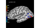
Source localization with MNE, dSPM, sLORETA, and eLORETA
The role of dipole orientations in distributed source localization
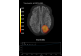
EEG source localization given electrode locations on an MRI
Working with CTF data: the Brainstorm auditory dataset
Preprocessing optically pumped magnetometer (OPM) MEG data