Note
Go to the end to download the full example code.
Visualize source time courses (stcs)#
This tutorial focuses on visualization of source estimates.
Surface Source Estimates#
First, we get the paths for the evoked data and the source time courses (stcs).
# Authors: The MNE-Python contributors.
# License: BSD-3-Clause
# Copyright the MNE-Python contributors.
import matplotlib.pyplot as plt
import numpy as np

import mne
from mne import read_evokeds
from mne.datasets import fetch_hcp_mmp_parcellation, sample
from mne.minimum_norm import apply_inverse, read_inverse_operator

data_path = sample.data_path()
meg_path = data_path / "MEG" / "sample"
subjects_dir = data_path / "subjects"

fname_evoked = meg_path / "sample_audvis-ave.fif"
fname_stc = meg_path / "sample_audvis-meg"
fetch_hcp_mmp_parcellation(subjects_dir)
Then, we read the stc from file.
stc = mne.read_source_estimate(fname_stc, subject="sample")
This is a SourceEstimate object.
print(stc)
<SourceEstimate | 7498 vertices, subject : sample, tmin : 0.0 (ms), tmax : 240.0 (ms), tstep : 10.0 (ms), data shape : (7498, 25), ~791 KiB>
The SourceEstimate object is in fact a surface source estimate. MNE also supports volume-based source estimates but more on that later.
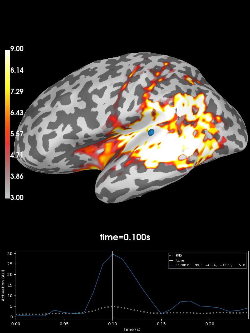
We can plot the source estimate using the
stc.plot just as in other MNE
objects. Note that for this visualization to work, you must have PyVista
installed on your machine.
initial_time = 0.1
brain = stc.plot(
    subjects_dir=subjects_dir,
    initial_time=initial_time,
    clim=dict(kind="value", lims=[3, 6, 9]),
    smoothing_steps=7,
)
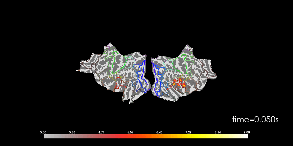
You can also morph it to fsaverage and visualize it using a flatmap.
stc_fs = mne.compute_source_morph(
    stc, "sample", "fsaverage", subjects_dir, smooth=5, verbose="error"
).apply(stc)
brain = stc_fs.plot(
    subjects_dir=subjects_dir,
    initial_time=initial_time,
    clim=dict(kind="value", lims=[3, 6, 9]),
    surface="flat",
    hemi="both",
    size=(1000, 500),
    smoothing_steps=5,
    time_viewer=False,
    add_data_kwargs=dict(colorbar_kwargs=dict(label_font_size=10)),
)

# to help orient us, let's add a parcellation (red=auditory, green=motor,
# blue=visual)
brain.add_annotation("HCPMMP1_combined", borders=2)

# You can save a movie like the one on our documentation website with:
# brain.save_movie(time_dilation=20, tmin=0.05, tmax=0.16,
#                  interpolation='linear', framerate=10)
Note that here we used initial_time=0.1, but we can also browse through
time using time_viewer=True.
In case PyVista is not available, we also offer a matplotlib
backend. Here we use verbose=’error’ to ignore a warning that not all
vertices were used in plotting.
mpl_fig = stc.plot(
    subjects_dir=subjects_dir,
    initial_time=initial_time,
    backend="matplotlib",
    verbose="error",
    smoothing_steps=7,
)
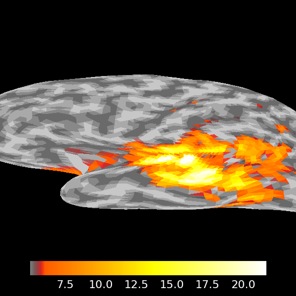
Volume Source Estimates#
We can also visualize volume source estimates (used for deep structures).
Let us load the sensor-level evoked data. We select the MEG channels to keep things simple.
evoked = read_evokeds(fname_evoked, condition=0, baseline=(None, 0))
evoked.pick(picks="meg").crop(0.05, 0.15)
# this risks aliasing, but these data are very smooth
evoked.decimate(10, verbose="error")
Reading /home/circleci/mne_data/MNE-sample-data/MEG/sample/sample_audvis-ave.fif ...
    Read a total of 4 projection items:
        PCA-v1 (1 x 10²) active
        PCA-v2 (1 x 10²) active
        PCA-v3 (1 x 10²) active
        Average EEG reference (1 x 60) active
    Found the data of interest:
        t =    -199.80 ...     499.49 ms (Left Auditory)
        0 CTF compensation matrices available
        nave = 55 - aspect type = 100
Projections have already been applied. Setting proj attribute to True.
Applying baseline correction (mode: mean)
Then, we can load the precomputed inverse operator from a file.
Reading inverse operator decomposition from /home/circleci/mne_data/MNE-sample-data/MEG/sample/sample_audvis-meg-vol-7-meg-inv.fif...
    Reading inverse operator info...
    [done]
    Reading inverse operator decomposition...
    [done]
    305 x 305 full covariance (kind = 1) found.
    Read a total of 4 projection items:
        PCA-v1 (1 x 10²) active
        PCA-v2 (1 x 10²) active
        PCA-v3 (1 x 10²) active
        Average EEG reference (1 x 60) active
    Noise covariance matrix read.
    11271 x 11271 diagonal covariance (kind = 2) found.
    Source covariance matrix read.
    Did not find the desired covariance matrix (kind = 6)
    11271 x 11271 diagonal covariance (kind = 5) found.
    Depth priors read.
    Did not find the desired covariance matrix (kind = 3)
    Reading a source space...
    [done]
    1 source spaces read
    Read a total of 4 projection items:
        PCA-v1 (1 x 10²) active
        PCA-v2 (1 x 10²) active
        PCA-v3 (1 x 10²) active
        Average EEG reference (1 x 60) active
    Source spaces transformed to the inverse solution coordinate frame
The source estimate is computed using the inverse operator and the sensor-space data.
Preparing the inverse operator for use...
    Scaled noise and source covariance from nave = 1 to nave = 55
    Created the regularized inverter
    Created an SSP operator (subspace dimension = 3)
    Created the whitener using a noise covariance matrix with rank 302 (3 small eigenvalues omitted)
    Computing noise-normalization factors (dSPM)...
[done]
Applying inverse operator to "Left Auditory"...
    Picked 305 channels from the data
    Computing inverse...
    Eigenleads need to be weighted ...
    Computing residual...
    Explained  77.1% variance
    Combining the current components...
    dSPM...
[done]
This time, we have a different container
(VolSourceEstimate) for the source time
course.
print(stc)
<VolSourceEstimate | 3757 vertices, subject : sample, tmin : 49.94880328959697 (ms), tmax : 149.84640986879091 (ms), tstep : 16.649601096532322 (ms), data shape : (3757, 7), ~235 KiB>
This too comes with a convenient plot method.
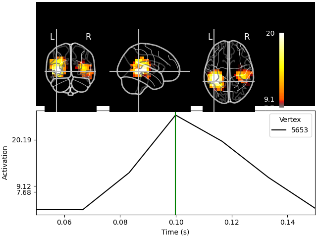
stc.plot(src, subject="sample", subjects_dir=subjects_dir)
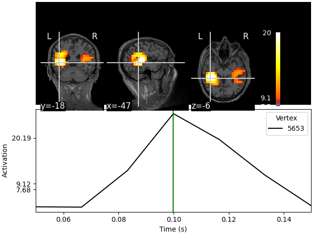
Showing: t = 0.100 s, (-47.3, -19.0, -6.3) mm, [4, 9, 10] vox, 5653 vertex
Using control points [ 7.67635542  9.11717401 20.19136023]
For this visualization, nilearn must be installed.
This visualization is interactive. Click on any of the anatomical slices
to explore the time series. Clicking on any time point will bring up the
corresponding anatomical map.
We could visualize the source estimate on a glass brain. Unlike the previous visualization, a glass brain does not show us one slice but what we would see if the brain was transparent like glass, and maximum intensity projection) is used:
stc.plot(src, subject="sample", subjects_dir=subjects_dir, mode="glass_brain")
Transforming subject RAS (non-zero origin) -> MNI Talairach
    1.022485 -0.008449 -0.036217       5.60 mm
    0.071071 0.914866 0.406098     -19.82 mm
    0.008756 -0.433700 1.028119      -1.55 mm
    0.000000 0.000000 0.000000       1.00

Showing: t = 0.100 s, (-42.4, -43.1, -0.2) mm, [4, 9, 10] vox, 5653 vertex
Using control points [ 7.67635542  9.11717401 20.19136023]
You can also extract label time courses using volumetric atlases. Here we’ll
use the built-in aparc+aseg.mgz:
fname_aseg = subjects_dir / "sample" / "mri" / "aparc+aseg.mgz"
label_names = mne.get_volume_labels_from_aseg(fname_aseg)
label_tc = stc.extract_label_time_course(fname_aseg, src=src)

lidx, tidx = np.unravel_index(np.argmax(label_tc), label_tc.shape)
fig, ax = plt.subplots(1, layout="constrained")
ax.plot(stc.times, label_tc.T, "k", lw=1.0, alpha=0.5)
xy = np.array([stc.times[tidx], label_tc[lidx, tidx]])
xytext = xy + [0.01, 1]
ax.annotate(label_names[lidx], xy, xytext, arrowprops=dict(arrowstyle="->"), color="r")
ax.set(xlim=stc.times[[0, -1]], xlabel="Time (s)", ylabel="Activation")
for key in ("right", "top"):
    ax.spines[key].set_visible(False)
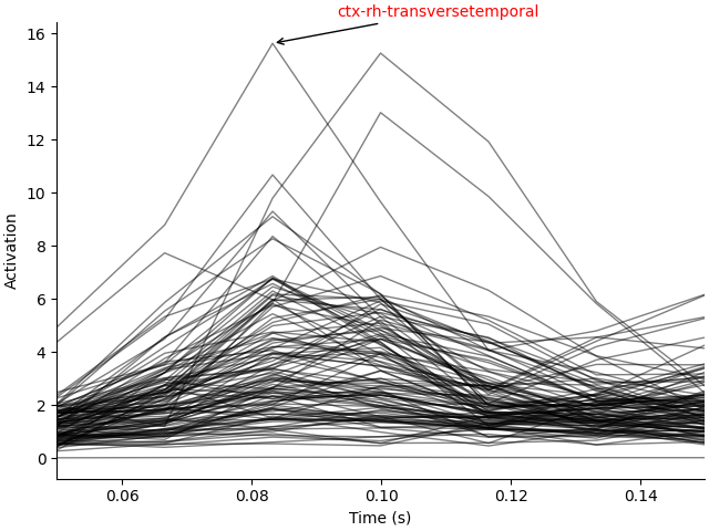
Reading atlas /home/circleci/mne_data/MNE-sample-data/subjects/sample/mri/aparc+aseg.mgz
114/114 atlas regions had at least one vertex in the source space
Extracting time courses for 114 labels (mode: mean)
We can plot several labels with the most activation in their time course for a more fine-grained view of the anatomical loci of activation.
labels = [
    label_names[idx]
    for idx in np.argsort(label_tc.max(axis=1))[:7]
    if "unknown" not in label_names[idx].lower()
]  # remove catch-all
brain = mne.viz.Brain(
    "sample",
    hemi="both",
    surf="pial",
    alpha=0.5,
    cortex="low_contrast",
    subjects_dir=subjects_dir,
)
brain.add_volume_labels(aseg="aparc+aseg", labels=labels)
brain.show_view(azimuth=250, elevation=40, distance=400)
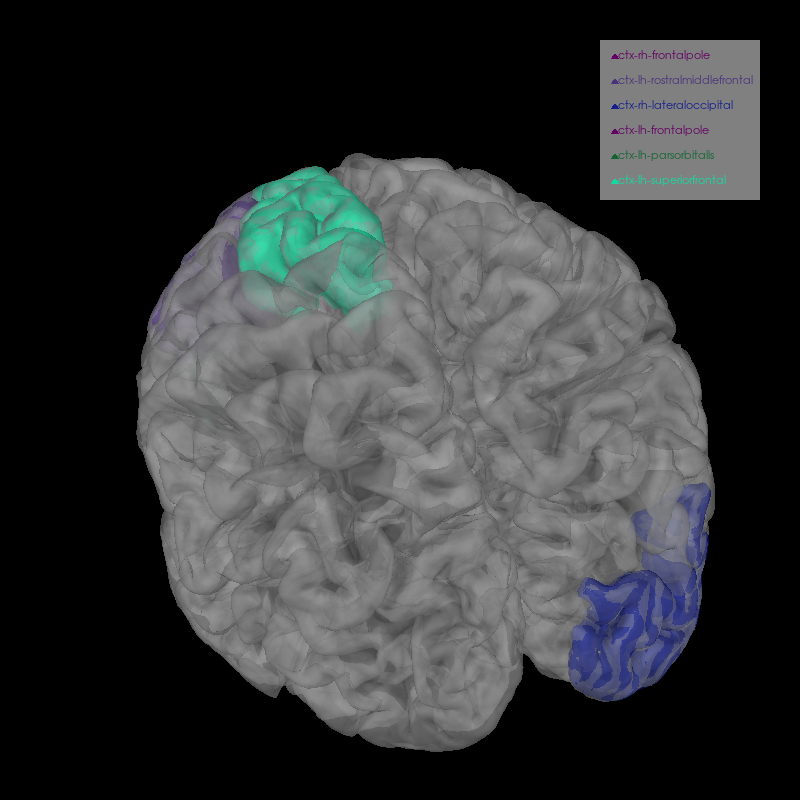
Smoothing by a factor of 0.9
And we can project these label time courses back to their original locations and see how the plot has been smoothed:
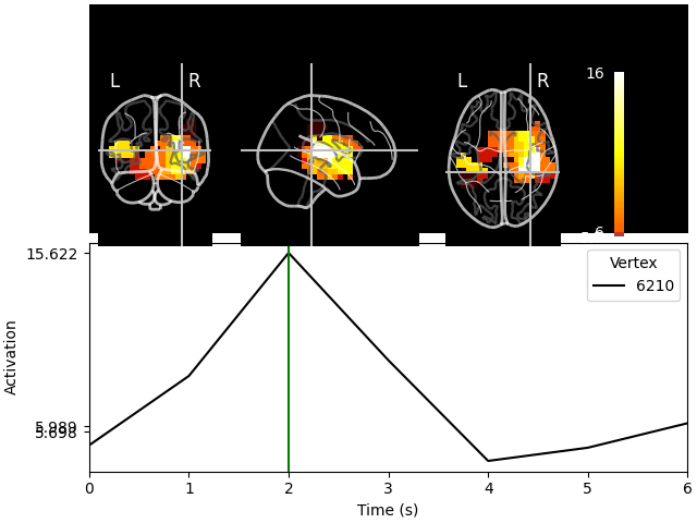
stc_back = mne.labels_to_stc(fname_aseg, label_tc, src=src)
stc_back.plot(src, subjects_dir=subjects_dir, mode="glass_brain")
Reading atlas /home/circleci/mne_data/MNE-sample-data/subjects/sample/mri/aparc+aseg.mgz
114/114 atlas regions had at least one vertex in the source space
Extracting time courses for 114 labels (mode: mean)
Transforming subject RAS (non-zero origin) -> MNI Talairach
    1.022485 -0.008449 -0.036217       5.60 mm
    0.071071 0.914866 0.406098     -19.82 mm
    0.008756 -0.433700 1.028119      -1.55 mm
    0.000000 0.000000 0.000000       1.00

Showing: t = 2.000 s, (36.1, -34.8, 7.7) mm, [15, 9, 11] vox, 6210 vertex
Using control points [ 5.69834054  5.98871778 15.62206532]
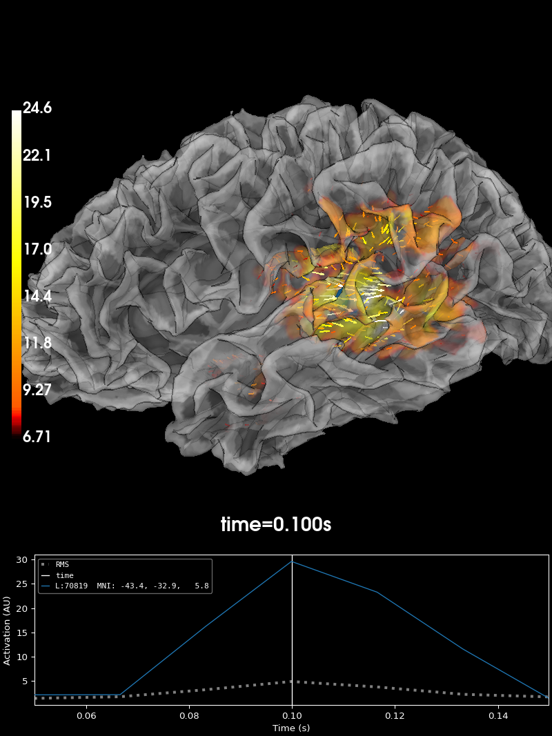
Vector Source Estimates#
If we choose to use pick_ori='vector' in
apply_inverse
fname_inv = data_path / "MEG" / "sample" / "sample_audvis-meg-oct-6-meg-inv.fif"
inv = read_inverse_operator(fname_inv)
stc = apply_inverse(evoked, inv, lambda2, "dSPM", pick_ori="vector")
brain = stc.plot(
    subject="sample",
    subjects_dir=subjects_dir,
    initial_time=initial_time,
    brain_kwargs=dict(silhouette=True),
    smoothing_steps=7,
)
Reading inverse operator decomposition from /home/circleci/mne_data/MNE-sample-data/MEG/sample/sample_audvis-meg-oct-6-meg-inv.fif...
    Reading inverse operator info...
    [done]
    Reading inverse operator decomposition...
    [done]
    305 x 305 full covariance (kind = 1) found.
    Read a total of 4 projection items:
        PCA-v1 (1 x 10²) active
        PCA-v2 (1 x 10²) active
        PCA-v3 (1 x 10²) active
        Average EEG reference (1 x 60) active
    Noise covariance matrix read.
    22494 x 22494 diagonal covariance (kind = 2) found.
    Source covariance matrix read.
    22494 x 22494 diagonal covariance (kind = 6) found.
    Orientation priors read.
    22494 x 22494 diagonal covariance (kind = 5) found.
    Depth priors read.
    Did not find the desired covariance matrix (kind = 3)
    Reading a source space...
    Computing patch statistics...
    Patch information added...
    Distance information added...
    [done]
    Reading a source space...
    Computing patch statistics...
    Patch information added...
    Distance information added...
    [done]
    2 source spaces read
    Read a total of 4 projection items:
        PCA-v1 (1 x 10²) active
        PCA-v2 (1 x 10²) active
        PCA-v3 (1 x 10²) active
        Average EEG reference (1 x 60) active
    Source spaces transformed to the inverse solution coordinate frame
Preparing the inverse operator for use...
    Scaled noise and source covariance from nave = 1 to nave = 55
    Created the regularized inverter
    Created an SSP operator (subspace dimension = 3)
    Created the whitener using a noise covariance matrix with rank 302 (3 small eigenvalues omitted)
    Computing noise-normalization factors (dSPM)...
[done]
Applying inverse operator to "Left Auditory"...
    Picked 305 channels from the data
    Computing inverse...
    Eigenleads need to be weighted ...
    Computing residual...
    Explained  77.5% variance
    dSPM...
[done]
Using control points [ 6.70708526  8.36619556 24.64056812]
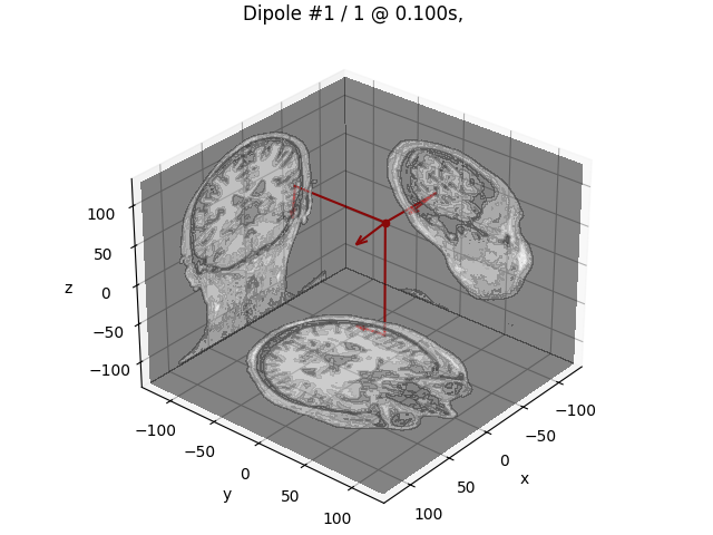
Dipole fits#
For computing a dipole fit, we need to load the noise covariance, the BEM solution, and the coregistration transformation files. Note that for the other methods, these were already used to generate the inverse operator.
fname_cov = meg_path / "sample_audvis-cov.fif"
fname_bem = subjects_dir / "sample" / "bem" / "sample-5120-bem-sol.fif"
fname_trans = meg_path / "sample_audvis_raw-trans.fif"
Dipoles are fit independently for each time point, so let us crop our time series to visualize the dipole fit for the time point of interest.
evoked.crop(0.1, 0.1)
dip = mne.fit_dipole(evoked, fname_cov, fname_bem, fname_trans)[0]
BEM               : PosixPath('/home/circleci/mne_data/MNE-sample-data/subjects/sample/bem/sample-5120-bem-sol.fif')
MRI transform     : /home/circleci/mne_data/MNE-sample-data/MEG/sample/sample_audvis_raw-trans.fif
Head origin       :   -4.2   19.3   65.3 mm rad =   72.3 mm.
Guess grid        :   20.0 mm
Guess mindist     :    5.0 mm
Guess exclude     :   20.0 mm
Using normal MEG coil definitions.
Noise covariance  : /home/circleci/mne_data/MNE-sample-data/MEG/sample/sample_audvis-cov.fif

Coordinate transformation: MRI (surface RAS) -> head
    0.999310 0.009985 -0.035787      -3.17 mm
    0.012759 0.812405 0.582954       6.86 mm
    0.034894 -0.583008 0.811716      28.88 mm
    0.000000 0.000000 0.000000       1.00
Coordinate transformation: MEG device -> head
    0.991420 -0.039936 -0.124467      -6.13 mm
    0.060661 0.984012 0.167456       0.06 mm
    0.115790 -0.173570 0.977991      64.74 mm
    0.000000 0.000000 0.000000       1.00
1 bad channels total
Read 305 MEG channels from info
105 coil definitions read
Coordinate transformation: MEG device -> head
    0.991420 -0.039936 -0.124467      -6.13 mm
    0.060661 0.984012 0.167456       0.06 mm
    0.115790 -0.173570 0.977991      64.74 mm
    0.000000 0.000000 0.000000       1.00
MEG coil definitions created in head coordinates.
Decomposing the sensor noise covariance matrix...
    Created an SSP operator (subspace dimension = 3)
Computing rank from covariance with rank=None
    Using tolerance 3.3e-13 (2.2e-16 eps * 305 dim * 4.8  max singular value)
    Estimated rank (mag + grad): 302
    MEG: rank 302 computed from 305 data channels with 3 projectors
    Setting small MEG eigenvalues to zero (without PCA)
    Created the whitener using a noise covariance matrix with rank 302 (3 small eigenvalues omitted)

---- Computing the forward solution for the guesses...
Guess surface (inner skull) is in MRI (surface RAS) coordinates
Filtering (grid =     20 mm)...
Surface CM = (   0.7  -10.0   44.3) mm
Surface fits inside a sphere with radius   91.8 mm
Surface extent:
    x =  -66.7 ...   68.8 mm
    y =  -88.0 ...   79.0 mm
    z =  -44.5 ...  105.8 mm
Grid extent:
    x =  -80.0 ...   80.0 mm
    y = -100.0 ...   80.0 mm
    z =  -60.0 ...  120.0 mm
900 sources before omitting any.
396 sources after omitting infeasible sources not within 20.0 - 91.8 mm.
Source spaces are in MRI coordinates.
Checking that the sources are inside the surface and at least    5.0 mm away (will take a few...)
Checking surface interior status for 396 points...
    Found  42/396 points inside  an interior sphere of radius   43.6 mm
    Found   0/396 points outside an exterior sphere of radius   91.8 mm
    Found 186/354 points outside using surface Qhull
    Found   9/168 points outside using solid angles
    Total 201/396 points inside the surface
Interior check completed in 230.5 ms
    195 source space points omitted because they are outside the inner skull surface.
    45 source space points omitted because of the    5.0-mm distance limit.
156 sources remaining after excluding the sources outside the surface and less than    5.0 mm inside.
Go through all guess source locations...
[done 156 sources]
---- Fitted :    99.9 ms, distance to inner skull : 7.6207 mm
Projections have already been applied. Setting proj attribute to True.
1 time points fitted
Finally, we can visualize the dipole.
dip.plot_locations(fname_trans, "sample", subjects_dir)
Total running time of the script: (1 minutes 9.158 seconds)