Note
Go to the end to download the full example code.
Creating MNE-Python data structures from scratch#
This tutorial shows how to create MNE-Python’s core data structures using an
existing NumPy array of (real or synthetic) data.
We begin by importing the necessary Python modules:
# Authors: The MNE-Python contributors.
# License: BSD-3-Clause
# Copyright the MNE-Python contributors.
import numpy as np

import mne
Creating Info objects#
The core data structures for continuous (Raw), discontinuous
(Epochs), and averaged (Evoked) data all have an info
attribute comprising an mne.Info object. When reading recorded data using
one of the functions in the mne.io submodule, Info objects are
created and populated automatically. But if we want to create a
Raw, Epochs, or Evoked object from scratch, we need
to create an appropriate Info object as well. The easiest way to do
this is with the mne.create_info function to initialize the required info
fields. Additional fields can be assigned later as one would with a regular
dictionary.
To initialize a minimal Info object requires a list of channel names,
and the sampling frequency. As a convenience for simulated data, channel
names can be provided as a single integer, and the names will be
automatically created as sequential integers (starting with 0):
# Create some dummy metadata
n_channels = 32
sampling_freq = 200  # in Hertz
info = mne.create_info(n_channels, sfreq=sampling_freq)
print(info)
<Info | 7 non-empty values
 bads: []
 ch_names: 0, 1, 2, 3, 4, 5, 6, 7, 8, 9, 10, 11, 12, 13, 14, 15, 16, 17, ...
 chs: 32 misc
 custom_ref_applied: False
 highpass: 0.0 Hz
 lowpass: 100.0 Hz
 meas_date: unspecified
 nchan: 32
 projs: []
 sfreq: 200.0 Hz
>
You can see in the output above that, by default, the channels are assigned
as type “misc” (where it says chs: 32 MISC). You can assign the channel
type when initializing the Info object if you want:
ch_names = [f"MEG{n:03}" for n in range(1, 10)] + ["EOG001"]
ch_types = ["mag", "grad", "grad"] * 3 + ["eog"]
info = mne.create_info(ch_names, ch_types=ch_types, sfreq=sampling_freq)
print(info)
<Info | 7 non-empty values
 bads: []
 ch_names: MEG001, MEG002, MEG003, MEG004, MEG005, MEG006, MEG007, MEG008, ...
 chs: 3 Magnetometers, 6 Gradiometers, 1 EOG
 custom_ref_applied: False
 highpass: 0.0 Hz
 lowpass: 100.0 Hz
 meas_date: unspecified
 nchan: 10
 projs: []
 sfreq: 200.0 Hz
>
If the channel names follow one of the standard montage naming schemes, their
spatial locations can be automatically added using the
set_montage method:
ch_names = ["Fp1", "Fp2", "Fz", "Cz", "Pz", "O1", "O2"]
ch_types = ["eeg"] * 7
info = mne.create_info(ch_names, ch_types=ch_types, sfreq=sampling_freq)
info.set_montage("standard_1020")
Note the new field dig that includes our seven channel locations as well
as theoretical values for the three
cardinal scalp landmarks.
Additional fields can be added in the same way that Python dictionaries are modified, using square-bracket key assignment:
<Info | 10 non-empty values
 bads: 1 items (O1)
 ch_names: Fp1, Fp2, Fz, Cz, Pz, O1, O2
 chs: 7 EEG
 custom_ref_applied: False
 description: My custom dataset
 dig: 10 items (3 Cardinal, 7 EEG)
 highpass: 0.0 Hz
 lowpass: 100.0 Hz
 meas_date: unspecified
 nchan: 7
 projs: []
 sfreq: 200.0 Hz
>
Creating Raw objects#
To create a Raw object from scratch, you can use the
mne.io.RawArray class constructor, which takes an Info object and a
NumPy array of shape (n_channels, n_samples).
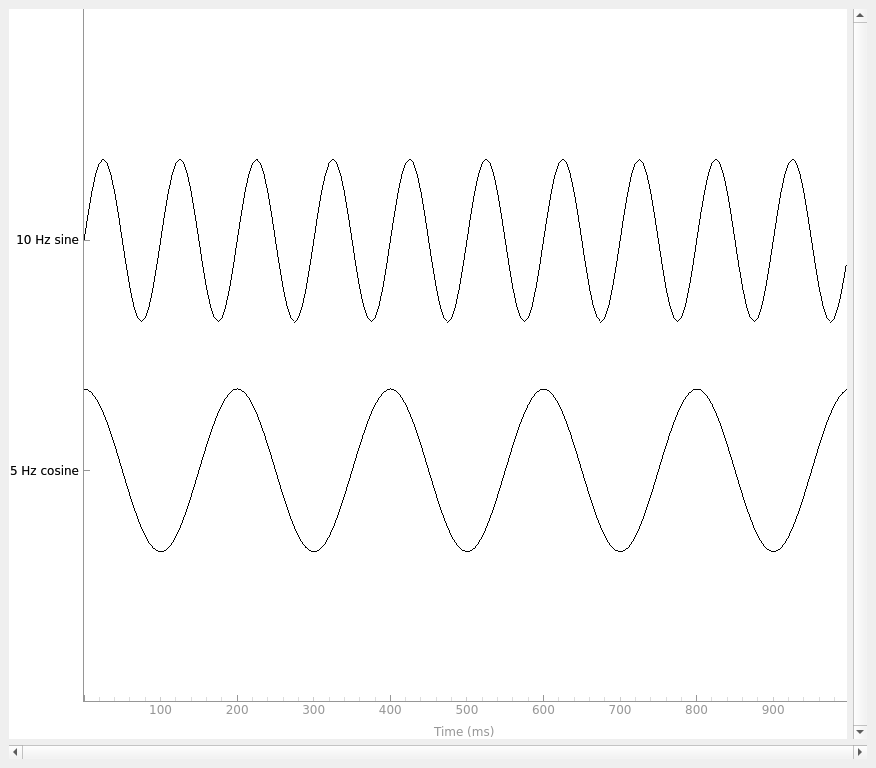
Here, we’ll create some sinusoidal data and plot it:
times = np.linspace(0, 1, sampling_freq, endpoint=False)
sine = np.sin(20 * np.pi * times)
cosine = np.cos(10 * np.pi * times)
data = np.array([sine, cosine])

info = mne.create_info(
    ch_names=["10 Hz sine", "5 Hz cosine"], ch_types=["misc"] * 2, sfreq=sampling_freq
)

simulated_raw = mne.io.RawArray(data, info)
simulated_raw.plot(show_scrollbars=False, show_scalebars=False)
Creating RawArray with float64 data, n_channels=2, n_times=200
    Range : 0 ... 199 =      0.000 ...     0.995 secs
Ready.
Using qt as 2D backend.
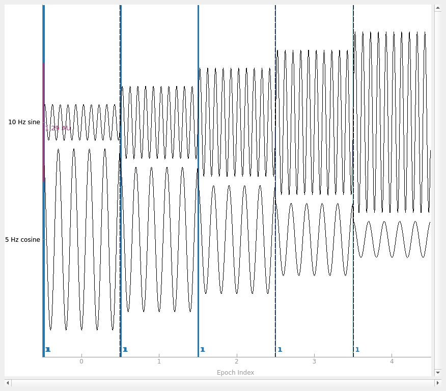
Creating Epochs objects#
To create an Epochs object from scratch, you can use the
mne.EpochsArray class constructor, which takes an Info object and a
NumPy array of shape (n_epochs, n_channels,
n_samples). Here we’ll create 5 epochs of our 2-channel data, and plot it.
Notice that we have to pass picks='misc' to the plot
method, because by default it only plots data channels.
Not setting metadata
5 matching events found
No baseline correction applied
0 projection items activated
You seem to have overlapping epochs. Some event lines may be duplicated in the plot.
Since we did not supply an events array, the EpochsArray constructor
automatically created one for us, with all epochs having the same event
number:
print(simulated_epochs.events[:, -1])
[1 1 1 1 1]
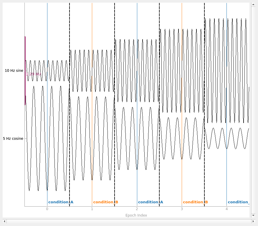
If we want to simulate having different experimental conditions, we can pass
an event array (and an event ID dictionary) to the constructor. Since our
epochs are 1 second long and have 200 samples/second, we’ll put our events
spaced 200 samples apart, and pass tmin=-0.5, so that the events
land in the middle of each epoch (the events are always placed at time=0 in
each epoch).
events = np.column_stack(
    (
        np.arange(0, 1000, sampling_freq),
        np.zeros(5, dtype=int),
        np.array([1, 2, 1, 2, 1]),
    )
)
event_dict = dict(condition_A=1, condition_B=2)
simulated_epochs = mne.EpochsArray(
    data, info, tmin=-0.5, events=events, event_id=event_dict
)
simulated_epochs.plot(
    picks="misc", show_scrollbars=False, events=events, event_id=event_dict
)
Not setting metadata
5 matching events found
No baseline correction applied
0 projection items activated
You could also create simulated epochs by using the normal Epochs
(not EpochsArray) constructor on the simulated RawArray
object, by creating an events array (e.g., using
mne.make_fixed_length_events) and extracting epochs around those events.
Creating Evoked Objects#
If you already have data that was averaged across trials, you can use it to
create an Evoked object using the EvokedArray class
constructor. It requires an Info object and a data array of shape
(n_channels, n_times), and has an optional tmin parameter like
EpochsArray does. It also has a parameter nave indicating how many
trials were averaged together, and a comment parameter useful for keeping
track of experimental conditions, etc. Here we’ll do the averaging on our
NumPy array and use the resulting averaged data to make our Evoked.
# Create the Evoked object
evoked_array = mne.EvokedArray(
    data.mean(axis=0), info, tmin=-0.5, nave=data.shape[0], comment="simulated"
)
print(evoked_array)
evoked_array.plot()
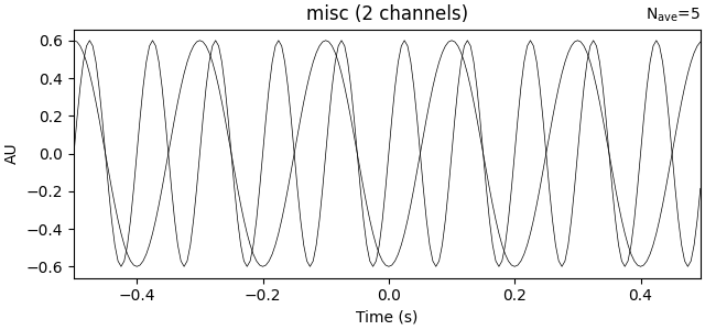
<Evoked | 'simulated' (average, N=5), -0.5 – 0.495 s, baseline off, 2 ch, ~9 KiB>
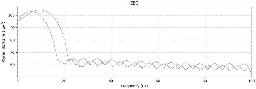
In certain situations you may wish to use a custom time-frequency
decomposition for estimation of power spectra. Or you may wish to
process pre-computed power spectra in MNE.
Following the same logic, it is possible to instantiate averaged power
spectrum using the SpectrumArray or
EpochsSpectrumArray classes.
# compute power spectrum

psd, freqs = mne.time_frequency.psd_array_welch(
    data, info["sfreq"], n_fft=128, n_per_seg=32
)

psd_ave = psd.mean(0)

info = mne.create_info(["Ch 1", "Ch2"], sfreq=sampling_freq, ch_types="eeg")
spectrum = mne.time_frequency.SpectrumArray(
    data=psd_ave,
    freqs=freqs,
    info=info,
)

spectrum.plot(spatial_colors=False, amplitude=False)
Effective window size : 0.640 (s)
Plotting power spectral density (dB=True).
Total running time of the script: (0 minutes 5.315 seconds)