Note
Go to the end to download the full example code.
Brainstorm CTF phantom dataset tutorial#
Here we compute the evoked from raw for the Brainstorm CTF phantom tutorial dataset. For comparison, see [1] and:
References#
# Authors: Eric Larson <larson.eric.d@gmail.com>
#
# License: BSD-3-Clause
# Copyright the MNE-Python contributors.
import warnings

import matplotlib.pyplot as plt
import numpy as np

import mne
from mne import fit_dipole
from mne.datasets.brainstorm import bst_phantom_ctf
from mne.io import read_raw_ctf

print(__doc__)
The data were collected with a CTF system at 2400 Hz.
data_path = bst_phantom_ctf.data_path(verbose=True)

# Switch to these to use the higher-SNR data:
# raw_path = op.join(data_path, 'phantom_200uA_20150709_01.ds')
# dip_freq = 7.
raw_path = data_path / "phantom_20uA_20150603_03.ds"
dip_freq = 23.0
erm_path = data_path / "emptyroom_20150709_01.ds"
raw = read_raw_ctf(raw_path, preload=True)
ds directory : /home/circleci/mne_data/MNE-brainstorm-data/bst_phantom_ctf/phantom_20uA_20150603_03.ds
    res4 data read.
    hc data read.
    Separate EEG position data file read.
    Quaternion matching (desired vs. transformed):
      -0.39   74.35    0.00 mm <->   -0.39   74.35   -0.00 mm (orig :  -39.23   63.82 -204.07 mm) diff =    0.000 mm
       0.39  -74.35    0.00 mm <->    0.39  -74.35    0.00 mm (orig :   65.69  -41.53 -205.68 mm) diff =    0.000 mm
      75.00    0.00    0.00 mm <->   75.00   -0.00    0.00 mm (orig :   64.32   61.80 -226.08 mm) diff =    0.000 mm
    Coordinate transformations established.
    Polhemus data for 3 HPI coils added
    Device coordinate locations for 3 HPI coils added
    Measurement info composed.
Finding samples for /home/circleci/mne_data/MNE-brainstorm-data/bst_phantom_ctf/phantom_20uA_20150603_03.ds/phantom_20uA_20150603_03.meg4:
    System clock channel is available, checking which samples are valid.
    10 x 2400 = 24000 samples from 304 chs
Current compensation grade : 3
Reading 0 ... 23999  =      0.000 ...    10.000 secs...
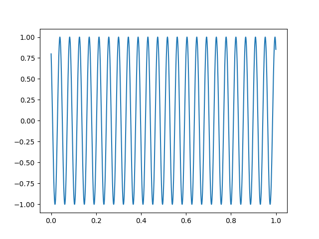
The sinusoidal signal is generated on channel HDAC006, so we can use that to obtain precise timing.
sinusoid, times = raw[raw.ch_names.index("HDAC006-4408")]
plt.figure()
plt.plot(times[times < 1.0], sinusoid.T[times < 1.0])
Let’s create some events using this signal by thresholding the sinusoid.
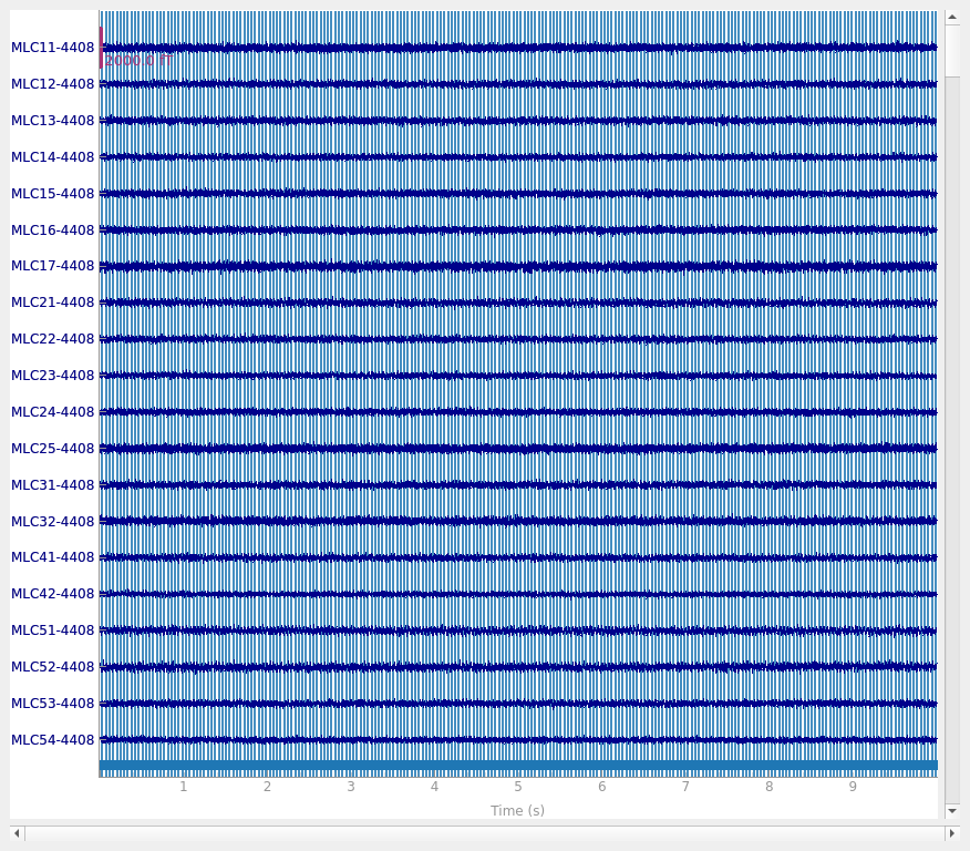
The CTF software compensation works reasonably well:
raw.plot()
Using qt as 2D backend.
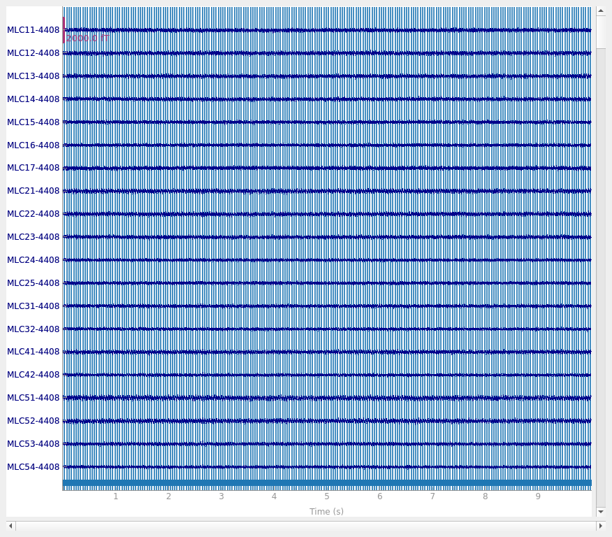
But here we can get slightly better noise suppression, lower localization bias, and a better dipole goodness of fit with spatio-temporal (tSSS) Maxwell filtering:
raw.apply_gradient_compensation(0)  # must un-do software compensation first
mf_kwargs = dict(origin=(0.0, 0.0, 0.0), st_duration=10.0, st_overlap=True)
raw = mne.preprocessing.maxwell_filter(raw, **mf_kwargs)
raw.plot()
Compensator constructed to change 3 -> 0
Applying compensator to loaded data
Maxwell filtering raw data
    No bad MEG channels
    Processing 0 gradiometers and 299 magnetometers (of which 290 are actually KIT gradiometers)
    Using origin 0.0, 0.0, 0.0 mm in the head frame
    Processing data using tSSS with st_duration=10.0
    Using loaded raw data
        Using 86/95 harmonic components for    0.000  (71/80 in, 15/15 out)
    Processing    1 data chunk of (at least) 10.0 s with 5.0 s overlap and hann windowing
        Using 86/95 harmonic components for    0.000  (71/80 in, 15/15 out)
        Projecting  8 intersecting tSSS components for    0.000 -   10.000 s
        Using 86/95 harmonic components for    0.000  (71/80 in, 15/15 out)
[done]
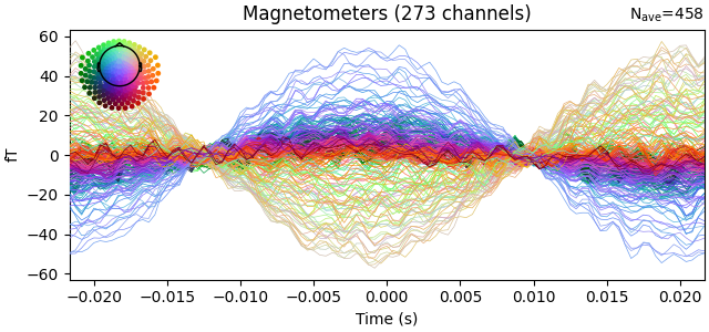
Our choice of tmin and tmax should capture exactly one cycle, so we can make the unusual choice of baselining using the entire epoch when creating our evoked data. We also then crop to a single time point (@t=0) because this is a peak in our signal.
tmin = -0.5 / dip_freq
tmax = -tmin
epochs = mne.Epochs(
    raw, events, event_id=1, tmin=tmin, tmax=tmax, baseline=(None, None)
)
evoked = epochs.average()
evoked.plot(time_unit="s")
evoked.crop(0.0, 0.0)
Not setting metadata
460 matching events found
Setting baseline interval to [-0.021666666666666667, 0.021666666666666667] s
Applying baseline correction (mode: mean)
0 projection items activated
Removing 5 compensators from info because not all compensation channels were picked.
Removing 5 compensators from info because not all compensation channels were picked.
Removing 5 compensators from info because not all compensation channels were picked.
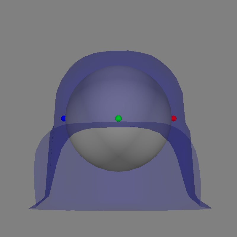
Let’s use a sphere head geometry model and let’s see the coordinate alignment and the sphere location.
sphere = mne.make_sphere_model(r0=(0.0, 0.0, 0.0), head_radius=0.08)

mne.viz.plot_alignment(
    raw.info, subject="sample", meg="helmet", bem=sphere, dig=True, surfaces=["brain"]
)
del raw, epochs
Equiv. model fitting -> RV = 0.00385873 %%
mu1 = 0.943736    lambda1 = 0.139585
mu2 = 0.66496    lambda2 = 0.685424
mu3 = -0.0416425    lambda3 = -0.0146395
Set up EEG sphere model with scalp radius    80.0 mm

Getting helmet for system CTF_275
To do a dipole fit, let’s use the covariance provided by the empty room recording.
raw_erm = read_raw_ctf(erm_path).apply_gradient_compensation(0)
raw_erm = mne.preprocessing.maxwell_filter(raw_erm, coord_frame="meg", **mf_kwargs)
cov = mne.compute_raw_covariance(raw_erm)
del raw_erm

with warnings.catch_warnings(record=True):
    # ignore warning about data rank exceeding that of info (75 > 71)
    warnings.simplefilter("ignore")
    dip, residual = fit_dipole(evoked, cov, sphere, verbose=True)
ds directory : /home/circleci/mne_data/MNE-brainstorm-data/bst_phantom_ctf/emptyroom_20150709_01.ds
    res4 data read.
    hc data read.
    Separate EEG position data file read.
    Quaternion matching (desired vs. transformed):
      -0.00   74.50    0.00 mm <->   -0.00   74.50   -0.00 mm (orig :  -50.17   57.61 -188.51 mm) diff =    0.000 mm
       0.00  -74.50    0.00 mm <->    0.00  -74.50    0.00 mm (orig :   60.49  -42.15 -190.81 mm) diff =    0.000 mm
      74.66    0.00    0.00 mm <->   74.66   -0.00    0.00 mm (orig :   53.03   61.29 -209.99 mm) diff =    0.000 mm
    Coordinate transformations established.
    Polhemus data for 3 HPI coils added
    Device coordinate locations for 3 HPI coils added
    Measurement info composed.
Finding samples for /home/circleci/mne_data/MNE-brainstorm-data/bst_phantom_ctf/emptyroom_20150709_01.ds/emptyroom_20150709_01.meg4:
    System clock channel is available, checking which samples are valid.
    100 x 600 = 60000 samples from 304 chs
Current compensation grade : 3
Compensator constructed to change 3 -> 0
Maxwell filtering raw data
    No bad MEG channels
    Processing 0 gradiometers and 299 magnetometers (of which 290 are actually KIT gradiometers)
    Using origin 0.0, 0.0, 0.0 mm in the meg frame (1.3, -8.8, -2.8 mm in the head frame)
    Processing data using tSSS with st_duration=10.0
    Loading raw data from disk
        Using 90/95 harmonic components for    0.000  (75/80 in, 15/15 out)
    Processing   19 data chunks of (at least) 10.0 s with 5.0 s overlap and hann windowing
        Using 90/95 harmonic components for    0.000  (75/80 in, 15/15 out)
        Projecting  8 intersecting tSSS components for    0.000 -    9.998 s
        Projecting  8 intersecting tSSS components for    5.000 -   14.998 s
        Projecting  8 intersecting tSSS components for   10.000 -   19.998 s
        Projecting  8 intersecting tSSS components for   15.000 -   24.998 s
        Projecting  8 intersecting tSSS components for   20.000 -   29.998 s
        Projecting  8 intersecting tSSS components for   25.000 -   34.998 s
        Projecting  8 intersecting tSSS components for   30.000 -   39.998 s
        Projecting  8 intersecting tSSS components for   35.000 -   44.998 s
        Projecting  9 intersecting tSSS components for   40.000 -   49.998 s
        Projecting  9 intersecting tSSS components for   45.000 -   54.998 s
        Projecting  8 intersecting tSSS components for   50.000 -   59.998 s
        Projecting  8 intersecting tSSS components for   55.000 -   64.998 s
        Projecting  7 intersecting tSSS components for   60.000 -   69.998 s
        Projecting  8 intersecting tSSS components for   65.000 -   74.998 s
        Projecting  9 intersecting tSSS components for   70.000 -   79.998 s
        Projecting  8 intersecting tSSS components for   75.000 -   84.998 s
        Projecting  9 intersecting tSSS components for   80.000 -   89.998 s
        Projecting  9 intersecting tSSS components for   85.000 -   94.998 s
        Projecting  8 intersecting tSSS components for   90.000 -   99.998 s
        Using 90/95 harmonic components for    0.000  (75/80 in, 15/15 out)
[done]
Using up to 500 segments
Number of samples used : 60000
[done]
BEM               : <ConductorModel | Sphere (3 layers): r0=[0.0, 0.0, 0.0] R=80 mm>
MRI transform     : identity
Sphere model      : origin at (   0.00    0.00    0.00) mm, rad =    0.1 mm
Guess grid        :   20.0 mm
Guess mindist     :    5.0 mm
Guess exclude     :   20.0 mm
Using normal MEG coil definitions.
Noise covariance  : <Covariance | kind : full, shape : (273, 273), range : [-4.1e-28, +1.2e-27], n_samples : 59999>

Coordinate transformation: MRI (surface RAS) -> head
    1.000000 0.000000 0.000000       0.00 mm
    0.000000 1.000000 0.000000       0.00 mm
    0.000000 0.000000 1.000000       0.00 mm
    0.000000 0.000000 0.000000       1.00
Coordinate transformation: MEG device -> head
    0.999939 -0.002039 -0.010868      -2.00 mm
    -0.001115 0.959234 -0.282612     -20.74 mm
    0.011001 0.282607 0.959173       9.38 mm
    0.000000 0.000000 0.000000       1.00
0 bad channels total
Read 299 MEG channels from info
Read 26 MEG compensation channels from info
5 compensation data sets in info
Setting up compensation data...
    No compensation set. Nothing more to do.
105 coil definitions read
Coordinate transformation: MEG device -> head
    0.999939 -0.002039 -0.010868      -2.00 mm
    -0.001115 0.959234 -0.282612     -20.74 mm
    0.011001 0.282607 0.959173       9.38 mm
    0.000000 0.000000 0.000000       1.00
MEG coil definitions created in head coordinates.
Decomposing the sensor noise covariance matrix...
Removing 5 compensators from info because not all compensation channels were picked.
Computing rank from covariance with rank=None
    Using tolerance 1.9e-15 (2.2e-16 eps * 273 dim * 0.031  max singular value)
    Estimated rank (mag): 75
    MAG: rank 75 computed from 273 data channels with 0 projectors
    Setting small MAG eigenvalues to zero (without PCA)
    Created the whitener using a noise covariance matrix with rank 75 (198 small eigenvalues omitted)

---- Computing the forward solution for the guesses...
Making a spherical guess space with radius    72.0 mm...
Filtering (grid =     20 mm)...
Surface CM = (   0.0    0.0    0.0) mm
Surface fits inside a sphere with radius   72.0 mm
Surface extent:
    x =  -72.0 ...   72.0 mm
    y =  -72.0 ...   72.0 mm
    z =  -72.0 ...   72.0 mm
Grid extent:
    x =  -80.0 ...   80.0 mm
    y =  -80.0 ...   80.0 mm
    z =  -80.0 ...   80.0 mm
729 sources before omitting any.
178 sources after omitting infeasible sources not within 20.0 - 72.0 mm.
Source spaces are in MRI coordinates.
Checking that the sources are inside the surface and at least    5.0 mm away (will take a few...)
    8 source space point omitted because of the    5.0-mm distance limit.
170 sources remaining after excluding the sources outside the surface and less than    5.0 mm inside.
Go through all guess source locations...
[done 170 sources]
---- Fitted :     0.0 ms
No projector specified for this dataset. Please consider the method self.add_proj.
1 time points fitted
Compare the actual position with the estimated one.
expected_pos = np.array([18.0, 0.0, 49.0])
diff = np.sqrt(np.sum((dip.pos[0] * 1000 - expected_pos) ** 2))
print(f"Actual pos:     {np.array_str(expected_pos, precision=1)} mm")
print(f"Estimated pos:  {np.array_str(dip.pos[0] * 1000, precision=1)} mm")
print(f"Difference:     {diff:0.1f} mm")
print(f"Amplitude:      {1e9 * dip.amplitude[0]:0.1f} nAm")
print(f"GOF:            {dip.gof[0]:0.1f} %")
Actual pos:     [18.  0. 49.] mm
Estimated pos:  [18.5 -2.2 44.6] mm
Difference:     5.0 mm
Amplitude:      10.1 nAm
GOF:            96.4 %
Total running time of the script: (0 minutes 28.663 seconds)