Adaptive ASR with chunk updates

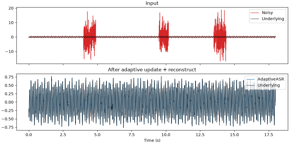
This example demonstrates the AASR-style adaptive update workflow. The calibration state is initialized on one chunk, updated on a second chunk, and then applied to the full signal with MATLAB-style reconstruct.

from __future__ import annotations

import matplotlib.pyplot as plt
import numpy as np

from mne_denoise.asr import AdaptiveASR

rng = np.random.default_rng(7)
sfreq = 250.0
duration = 18.0
n_times = int(sfreq * duration)
n_channels = 8
t = np.arange(n_times) / sfreq

brain = np.zeros((n_channels, n_times), dtype=np.float64)
for ch_idx in range(n_channels):
    phase = rng.uniform(0.0, 2.0 * np.pi)
    brain[ch_idx] = (
        0.5 * np.sin(2.0 * np.pi * 10.0 * t + phase)
        + 0.15 * np.sin(2.0 * np.pi * 6.0 * t + 0.5 * phase)
        + 0.05 * rng.standard_normal(n_times)
    )

data = brain.copy()
spatial = rng.standard_normal((n_channels, 2))
spatial /= np.linalg.norm(spatial, axis=0, keepdims=True)
for onset, stop in ((4.0, 4.9), (9.5, 10.2), (13.5, 14.4)):
    start = int(onset * sfreq)
    stop_samp = int(stop * sfreq)
    source = rng.standard_normal((2, stop_samp - start)) * 8.0
    data[:, start:stop_samp] += spatial @ source

chunk = int(6.0 * sfreq)
asr = AdaptiveASR(
    sfreq=sfreq,
    cutoff=20.0,
    variant="psw",
    verbose=False,
)
asr.fit(data[:, :chunk])
asr.partial_fit(data[:, chunk : 2 * chunk])
cleaned = asr.transform(data)

fig, axes = plt.subplots(2, 1, figsize=(10, 5), sharex=True, layout="constrained")
axes[0].plot(t, data[0], color="tab:red", lw=1.0, label="Noisy")
axes[0].plot(t, brain[0], color="k", lw=1.0, alpha=0.7, label="Underlying")
axes[0].set_title("Input")
axes[0].legend(loc="upper right")

axes[1].plot(t, cleaned[0], color="tab:blue", lw=1.0, label="AdaptiveASR")
axes[1].plot(t, brain[0], color="k", lw=1.0, alpha=0.7, label="Underlying")
axes[1].set_title("After adaptive update + reconstruct")
axes[1].set_xlabel("Time (s)")
axes[1].legend(loc="upper right")

plt.show()