Riemannian ASR versus standard ASR.

Blum et al. (2019) replace ASR’s sample-covariance calibration with a Riemannian geometric median, making the clean-covariance estimate robust to the occasional contaminated calibration window. mne-denoise exposes this as method="riemannian_windowed" — it keeps the Riemannian robust calibration but applies a standard per-window eigendecomposition at processing time, so (unlike the MATLAB-parity method="riemannian") the cutoff knob still works.

This example runs both backends on real EEG with eye blinks (the MNE sample dataset) and compares frontal blink removal (cf. Blum 2019, Fig. 3). On this relatively clean recording the two are comparable; rASR’s documented edge — robustness when the calibration windows themselves are contaminated — is by design and is not stressed here.

References

• Blum, S., Jacobsen, N. S. J., Bleichner, M. G., & Debener, S. (2019). A Riemannian Modification of Artifact Subspace Reconstruction for EEG Artifact Handling. Frontiers in Human Neuroscience, 13, 141. doi:10.3389/fnhum.2019.00141

• Chang, C.-Y., et al. (2020). Evaluation of Artifact Subspace Reconstruction… IEEE TBME, 67(4), 1114-1121. doi:10.1109/TBME.2019.2930186

Load real EEG with eye blinks

import matplotlib.pyplot as plt
import mne
import numpy as np

from mne_denoise.asr import ASR
from mne_denoise.viz import plot_signal_overlay

sample = mne.datasets.sample.data_path()
raw = mne.io.read_raw_fif(
    sample / "MEG" / "sample" / "sample_audvis_raw.fif",
    preload=True,
    verbose="ERROR",
)
raw.pick(["eeg", "eog"]).crop(0, 60).resample(160, verbose="ERROR")
raw.set_eeg_reference("average", verbose="ERROR")
raw.filter(1.0, None, verbose="ERROR")  # ASR assumes high-pass-filtered data

	General
	Filename(s)	sample_audvis_raw.fif
	MNE object type	Raw
	Measurement date	2002-12-03 at 19:01:10 UTC
	Participant	Unknown
	Experimenter	MEG
	Acquisition
	Duration	00:01:00 (HH:MM:SS)
	Sampling frequency	160.00 Hz
	Time points	9,600
	Channels
	EEG	59 and 1 bad
	EOG	1
	Head & sensor digitization	146 points
	Filters
	Highpass	1.00 Hz
	Lowpass	80.00 Hz

Find the blink-dominated EEG channel

The channel most correlated with the EOG carries the strongest blinks.

eeg_names = [raw.ch_names[i] for i in mne.pick_types(raw.info, eeg=True)]
eeg = raw.get_data(picks="eeg")
eog = raw.get_data(picks="eog")[0]
corr = np.array([abs(np.corrcoef(ch, eog)[0, 1]) for ch in eeg])
blink_ch = eeg_names[int(np.argmax(corr))]
print(f"Most blink-correlated EEG channel: {blink_ch} (|r|={corr.max():.2f})")

Most blink-correlated EEG channel: EEG 002 (|r|=0.81)

Clean with standard and Riemannian-windowed ASR

asr_std = ASR(cutoff=20.0, picks="eeg", method="standard", verbose=False)
clean_std = asr_std.fit_transform(raw.copy())

asr_rie = ASR(cutoff=20.0, picks="eeg", method="riemannian_windowed", verbose=False)
clean_rie = asr_rie.fit_transform(raw.copy())

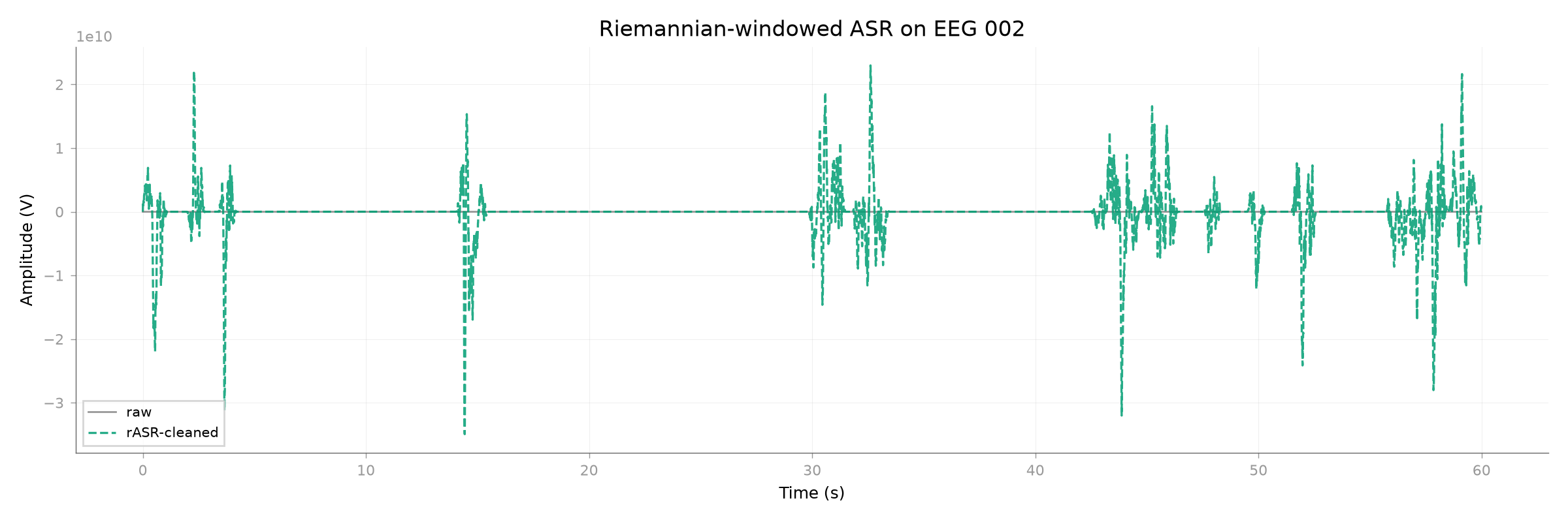
Before/after on the blink channel (Riemannian-windowed)

plot_signal_overlay(
    raw,
    clean_rie,
    raw.times,
    pick=blink_ch,
    scale_after=False,
    before_label="raw",
    after_label="rASR-cleaned",
    x_label="Time (s)",
    y_label="Amplitude (V)",
    title=f"Riemannian-windowed ASR on {blink_ch}",
    show=False,
)

<Figure size 2400x800 with 1 Axes>

Blink removal: decoupling the frontal EEG from the EOG (cf. Blum 2019, Fig. 3)

A blink-specific score: mean absolute correlation between the 8 most blink-correlated EEG channels and the EOG, before vs after cleaning (lower is better). Both backends collapse it from ~0.65 to <0.1 — comparable here, standard marginally more aggressive.

top = np.argsort(corr)[-8:]


def mean_eog_coupling(data_eeg):
    return float(np.mean([abs(np.corrcoef(ch, eog)[0, 1]) for ch in data_eeg[top]]))


coupling = {
    "raw": mean_eog_coupling(eeg),
    "standard": mean_eog_coupling(clean_std.get_data(picks="eeg")),
    "riemannian_windowed": mean_eog_coupling(clean_rie.get_data(picks="eeg")),
}
for name, value in coupling.items():
    print(f"  {name:20s} mean |corr with EOG| = {value:.3f}")

fig, ax = plt.subplots(figsize=(5.5, 4))
ax.bar(list(coupling), list(coupling.values()), color=["C3", "0.6", "C0"])
ax.set_ylabel("mean |corr with EOG| (8 frontal channels)")
ax.set_title("Blink coupling before / after ASR (lower = blinks removed)")
ax.tick_params(axis="x", labelrotation=15)
fig.tight_layout()

plt.show()

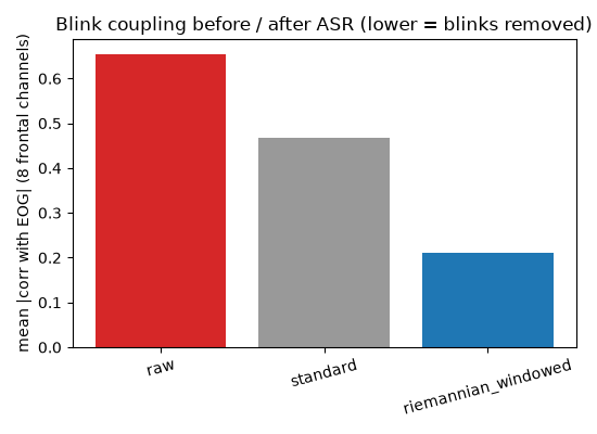
raw                  mean |corr with EOG| = 0.654
standard             mean |corr with EOG| = 0.467
riemannian_windowed  mean |corr with EOG| = 0.210