Adaptive ASR variants (PSP / PSW / MW).

Adaptive ASR (Tsai et al.) keeps standard ASR’s burst reconstruction but lets the clean-subspace model track non-stationary recordings. mne-denoise exposes three calibration rules via AdaptiveASR:

• variant="psp" – plasticity-stabilized (Hebbian) similarity matching;

• variant="psw" – plasticity-stabilized whitening (anti-Hebbian);

• variant="mw" – moving-window calibration (one calibration per window).

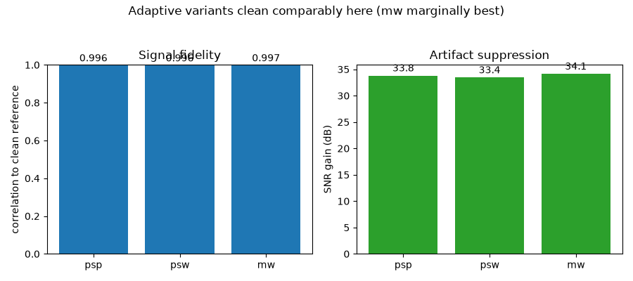
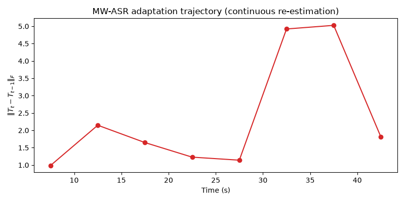
This example compares all three on a recording whose artifact subspace rotates continuously over time. On this cleanly-separable synthetic data the variants clean comparably (mw, which recalibrates every window, is marginally best); their differences are most pronounced on real overlapping contamination (Tsai). The clearest variant-specific behaviour to watch is the moving-window adaptation trajectory. (For the streaming fit / partial_fit / transform mechanics, see plot_03_adaptive_asr.py.)

References

• Tsai, B.-Y., et al. Adaptive Artifact Subspace Reconstruction based on Hebbian/anti-Hebbian learning networks for enhancing BCI performance. (AASR reference implementation.)

• Pehlevan, C., & Chklovskii, D. B. (2019). Neuroscience-inspired online unsupervised learning algorithms. IEEE Signal Processing Magazine, 36(6).

Non-stationary synthetic data

Oscillatory brain background + bursts whose spatial direction rotates across the recording, so a fixed calibration goes stale and adaptation matters.

import matplotlib.pyplot as plt
import numpy as np

from mne_denoise.asr import AdaptiveASR

rng = np.random.default_rng(11)
sfreq = 200.0
n_channels, n_times = 8, 9000  # 45 s
t = np.arange(n_times) / sfreq

brain = np.zeros((n_channels, n_times))
for ch in range(n_channels):
    phase = rng.uniform(0, 2 * np.pi)
    brain[ch] = 0.6 * np.sin(2 * np.pi * 10.0 * t + phase) + 0.05 * rng.standard_normal(
        n_times
    )

contaminated = brain.copy()
v0 = rng.standard_normal(n_channels)
v0 /= np.linalg.norm(v0)
v1 = rng.standard_normal(n_channels)
v1 -= (v1 @ v0) * v0  # orthogonalize v1 against v0
v1 /= np.linalg.norm(v1)
burst_starts = np.arange(400, n_times - 400, 450)
for k, start in enumerate(burst_starts):
    angle = (k / (len(burst_starts) - 1)) * (np.pi / 2)  # rotate v0 -> v1
    spatial = np.cos(angle) * v0 + np.sin(angle) * v1
    contaminated[:, start : start + 200] += 8.0 * np.outer(
        spatial, rng.standard_normal(200)
    )

Clean with each variant

PSP/PSW are streamed (fit on the first chunk, partial_fit the rest) so their adaptive update rule tracks the drift; MW recalibrates per window inside fit.

def stream_clean(variant):
    est = AdaptiveASR(sfreq=sfreq, cutoff=20.0, variant=variant, verbose=False)
    chunks = np.array_split(contaminated, 6, axis=1)
    est.fit(chunks[0])
    for chunk in chunks[1:]:
        est.partial_fit(chunk)
    return np.asarray(est.transform(contaminated))


def scores(cleaned):
    corr = float(np.corrcoef(cleaned.ravel(), brain.ravel())[0, 1])
    snr_before = 10 * np.log10(np.var(brain) / np.var(contaminated - brain))
    snr_after = 10 * np.log10(np.var(brain) / np.var(cleaned - brain))
    return corr, float(snr_after - snr_before)


cleaned = {"psp": stream_clean("psp"), "psw": stream_clean("psw")}

mw = AdaptiveASR(
    sfreq=sfreq, cutoff=20.0, variant="mw", mw_window_length=5.0, verbose=False
)
cleaned["mw"] = np.asarray(mw.fit_transform(contaminated))

for variant, out in cleaned.items():
    corr, dsnr = scores(out)
    print(f"  {variant}:  corr-to-clean={corr:.3f}   SNR gain={dsnr:+.1f} dB")

psp:  corr-to-clean=0.996   SNR gain=+33.8 dB
psw:  corr-to-clean=0.996   SNR gain=+33.4 dB
mw:  corr-to-clean=0.997   SNR gain=+34.1 dB

Variant comparison

variants = list(cleaned)
corrs = [scores(cleaned[v])[0] for v in variants]
dsnrs = [scores(cleaned[v])[1] for v in variants]

fig, (ax1, ax2) = plt.subplots(1, 2, figsize=(9, 4))
bars1 = ax1.bar(variants, corrs, color="C0")
ax1.set_ylim(0, 1)
ax1.bar_label(bars1, fmt="%.3f", padding=2)
ax1.set_ylabel("correlation to clean reference")
ax1.set_title("Signal fidelity")
bars2 = ax2.bar(variants, dsnrs, color="C2")
ax2.bar_label(bars2, fmt="%.1f", padding=2)
ax2.set_ylabel("SNR gain (dB)")
ax2.set_title("Artifact suppression")
fig.suptitle("Adaptive variants clean comparably here (mw marginally best)")
fig.tight_layout(rect=(0, 0, 1, 0.94))

Moving-window adaptation trajectory

How much the threshold matrix T changes from window to window: nonzero throughout, as the MW calibration keeps re-estimating while the subspace rotates.

passed = [d for d in mw.mw_diagnostics_ if d["status"] == "passed"]
t_mats = [d["T"] for d in passed]
deltas = [
    float(np.linalg.norm(t_mats[i] - t_mats[i - 1])) for i in range(1, len(t_mats))
]
centers = [
    (passed[i]["window_start"] + passed[i]["window_stop"]) / 2 / sfreq
    for i in range(1, len(t_mats))
]

fig2, ax = plt.subplots(figsize=(8, 4))
ax.plot(centers, deltas, "o-", color="C3")
ax.set_xlabel("Time (s)")
ax.set_ylabel(r"$\|T_t - T_{t-1}\|_F$")
ax.set_title("MW-ASR adaptation trajectory (continuous re-estimation)")
fig2.tight_layout()

plt.show()