Local SSA properties on a synthetic signal

This is an algorithm demonstration, not a replication of Teixeira et al.’s figures. The desired signal is broadband so that the example exercises the paper’s high-energy-structure-versus-residual assumption without constructing an unrealistically perfect separability case.

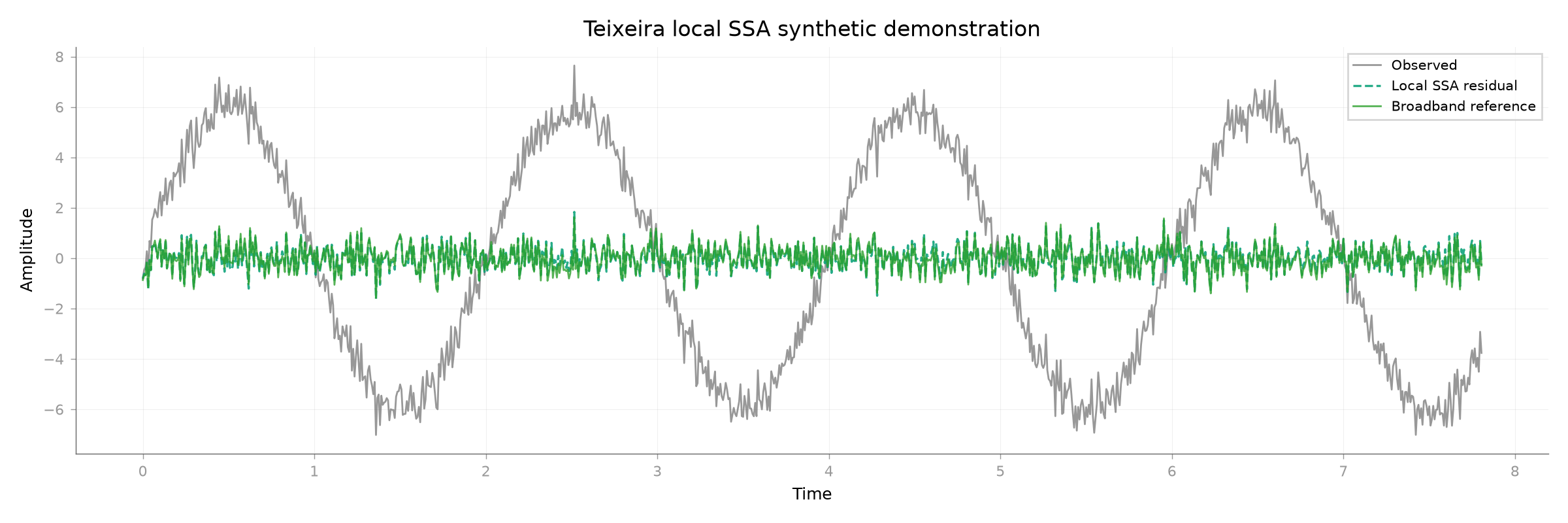
Correlation with broadband reference: 0.975
Reference gain: 0.941
MDL dimensions: [2 1 1 1 1 2]

<Figure size 2400x800 with 1 Axes>

import numpy as np

from mne_denoise.ssa import LocalSingularSpectrumAnalysis
from mne_denoise.viz import plot_signal_overlay

sfreq = 128.0
times = np.arange(1000) / sfreq
rng = np.random.default_rng(8)
neural = 0.5 * rng.standard_normal(times.size)
artifact = 6.0 * np.sin(2 * np.pi * 0.5 * times)
observed = neural + artifact + 0.05 * rng.standard_normal(times.size)

cleaner = LocalSingularSpectrumAnalysis(
    window_length=41,
    n_clusters=6,
    random_state=0,
)
cleaned = cleaner.fit_transform(observed[np.newaxis])[0]
correlation = np.corrcoef(cleaned, neural)[0, 1]
gain = np.dot(cleaned, neural) / np.dot(neural, neural)
print(f"Correlation with broadband reference: {correlation:.3f}")
print(f"Reference gain: {gain:.3f}")
print(f"MDL dimensions: {cleaner.subspace_dimensions_[0]}")

plot_signal_overlay(
    observed,
    cleaned,
    times,
    reference=neural,
    before_label="Observed",
    after_label="Local SSA residual",
    reference_label="Broadband reference",
    scale_after=False,
    title="Teixeira local SSA synthetic demonstration",
    show=False,
)