Juggler ASR: DBSCAN vs GEV reference selection.

On heavily contaminated recordings (mobile / MoBI EEG, dense brief bursts), ASR’s window-based clean-data selector starves — too few windows are clean enough to calibrate. Kim et al. (2025) instead select clean samples point-by-point. mne-denoise exposes two selectors via JugglerASR:

• strategy="dbscan" – density clustering of amplitude features (permissive);

• strategy="gev" – a Generalized-Extreme-Value tail fit (tighter).

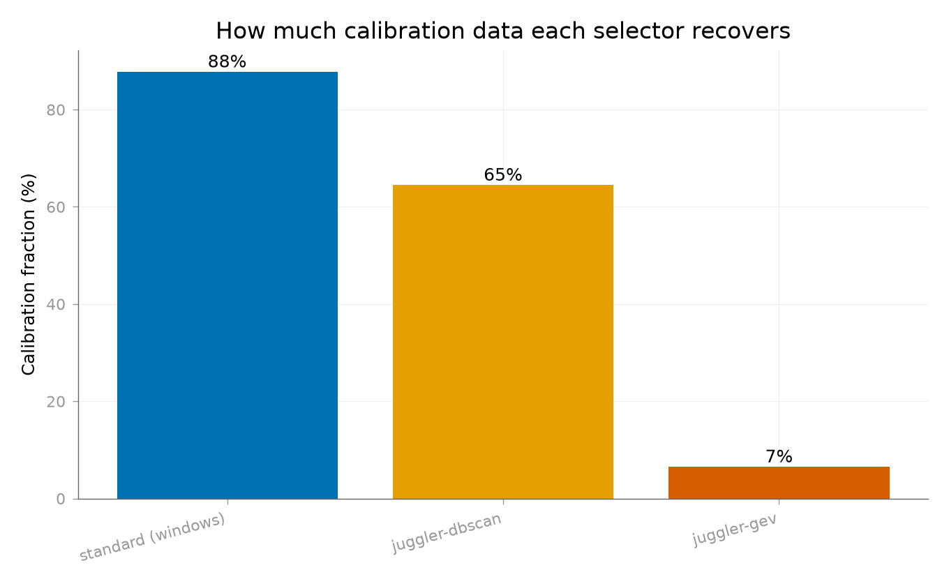
This example builds a densely-contaminated stream and compares how much calibration data each selector recovers, where the standard window selector struggles.

References

• Kim, S., et al. (2025). Juggler’s ASR: unpacking the principles of artifact subspace reconstruction for revision toward extreme MoBI. Journal of Neuroscience Methods, 420, 110465. doi:10.1016/j.jneumeth.2025.110465

Densely-contaminated synthetic data

Short bursts every ~0.4 s leave only small clean gaps – hard for a window-based selector, the regime Juggler targets.

import matplotlib.pyplot as plt
import numpy as np

from mne_denoise.asr import ASR, JugglerASR
from mne_denoise.viz import plot_asr_calibration_fraction

rng = np.random.default_rng(7)
sfreq = 250.0
n_channels, n_times = 12, 10000  # 40 s
t = np.arange(n_times) / sfreq

brain = np.zeros((n_channels, n_times))
for ch in range(n_channels):
    phase = rng.uniform(0, 2 * np.pi)
    brain[ch] = 0.6 * np.sin(2 * np.pi * 10.0 * t + phase) + 0.05 * rng.standard_normal(
        n_times
    )

contaminated = brain.copy()
burst_len = int(0.1 * sfreq)
for start in np.arange(300, n_times - burst_len, int(0.4 * sfreq)):
    spatial = rng.standard_normal(n_channels)
    spatial /= np.linalg.norm(spatial)
    contaminated[:, start : start + burst_len] += 9.0 * np.outer(
        spatial, rng.standard_normal(burst_len)
    )

Calibrate with the standard window selector and the two Juggler selectors

standard = ASR(sfreq=sfreq, cutoff=20.0, picks=None, verbose=False)
standard.fit_transform(contaminated)

dbscan = JugglerASR(
    sfreq=sfreq, cutoff=20.0, strategy="dbscan", picks=None, verbose=False
)
dbscan.fit_transform(contaminated)

gev = JugglerASR(sfreq=sfreq, cutoff=20.0, strategy="gev", picks=None, verbose=False)
gev.fit_transform(contaminated)

print(
    "reference fraction:  "
    f"dbscan={dbscan.calibration_info_['reference_selected_fraction']:.2f}  "
    f"gev={gev.calibration_info_['reference_selected_fraction']:.2f}"
)

reference fraction:  dbscan=0.65  gev=0.07

Calibration fraction across selectors

plot_asr_calibration_fraction(
    [standard, dbscan, gev],
    labels=["standard (windows)", "juggler-dbscan", "juggler-gev"],
    title="How much calibration data each selector recovers",
    show=False,
)

(<Figure size 1360x840 with 1 Axes>, <Axes: title={'center': 'How much calibration data each selector recovers'}, ylabel='Calibration fraction (%)'>)

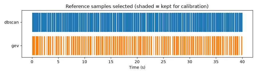
Reference-sample selection timeline (DBSCAN vs GEV)

Which individual samples each strategy trusts as clean reference, over time.

mask_db = dbscan.get_calibration_mask()
mask_gev = gev.get_calibration_mask()

fig, ax = plt.subplots(figsize=(9, 2.6))
ax.fill_between(t, 1.1, 1.9, where=mask_db, color="C0", step="mid", label="dbscan")
ax.fill_between(t, 0.1, 0.9, where=mask_gev, color="C1", step="mid", label="gev")
ax.set_yticks([0.5, 1.5])
ax.set_yticklabels(["gev", "dbscan"])
ax.set_xlabel("Time (s)")
ax.set_title("Reference samples selected (shaded = kept for calibration)")
ax.set_ylim(0, 2)
fig.tight_layout()

plt.show()