Choosing the ASR cutoff.

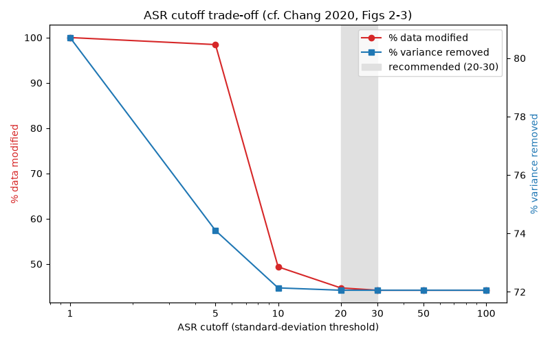
The ASR cutoff (standard-deviation threshold) is the single most important knob: lower values clean aggressively (and risk removing real high-variance brain activity), higher values are conservative. This example sweeps the cutoff and plots the two quantities Chang et al. (2020) use to characterise it — the fraction of data modified and the variance removed — reproducing the monotone trade-off of their Figs 2-3 and the commonly recommended 20-30 band.

References

• Chang, C.-Y., Hsu, S.-H., Pion-Tonachini, L., & Jung, T.-P. (2020). Evaluation of Artifact Subspace Reconstruction for Automatic Artifact Components Removal in Multi-Channel EEG Recordings. IEEE Transactions on Biomedical Engineering, 67(4), 1114-1121. doi:10.1109/TBME.2019.2930186

• Mullen, T. R., et al. (2013). Real-time modeling and 3D visualization of source dynamics and connectivity using wearable EEG. EMBC 2013. doi:10.1109/EMBC.2013.6609968

Imports and synthetic data

Oscillatory “brain” background plus spatially-structured high-amplitude bursts.

import matplotlib.pyplot as plt
import numpy as np

from mne_denoise.asr import ASR
from mne_denoise.qa import variance_removed

rng = np.random.default_rng(2024)
sfreq = 250.0
n_channels, n_times = 16, 12000  # 48 s
t = np.arange(n_times) / sfreq

brain = np.zeros((n_channels, n_times))
for ch in range(n_channels):
    phase = rng.uniform(0, 2 * np.pi)
    brain[ch] = (
        0.6 * np.sin(2 * np.pi * 10.0 * t + phase)
        + 0.15 * np.sin(2 * np.pi * 6.0 * t + 0.7 * phase)
        + 0.05 * rng.standard_normal(n_times)
    )

contaminated = brain.copy()
# Graded burst severities (1.5x -> 9x): aggressive cutoffs remove even the mild
# bursts, conservative cutoffs only the strongest -> both metrics vary with cutoff.
starts = np.linspace(800, n_times - 700, 12).astype(int)
amplitudes = np.linspace(1.5, 9.0, len(starts))
for start, amp in zip(starts, amplitudes):
    spatial = rng.standard_normal(n_channels)
    spatial /= np.linalg.norm(spatial)
    contaminated[:, start : start + 250] += amp * np.outer(
        spatial, rng.standard_normal(250)
    )

Sweep the cutoff

For each cutoff, fit + transform and read the two headline metrics straight from variance_removed().

cutoffs = [1, 5, 10, 20, 30, 50, 100]
pct_modified, pct_var_removed = [], []
for k in cutoffs:
    asr = ASR(sfreq=sfreq, cutoff=float(k), picks=None, verbose=False)
    cleaned = np.asarray(asr.fit_transform(contaminated))
    pct_modified.append(100.0 * asr.fraction_reconstructed_samples_)
    pct_var_removed.append(variance_removed(contaminated, cleaned))
    print(
        f"cutoff={k:3d}:  data modified={pct_modified[-1]:5.1f}%   "
        f"variance removed={pct_var_removed[-1]:5.1f}%"
    )

cutoff=  1:  data modified=100.0%   variance removed= 80.7%
cutoff=  5:  data modified= 98.5%   variance removed= 74.1%
cutoff= 10:  data modified= 49.4%   variance removed= 72.1%
cutoff= 20:  data modified= 44.7%   variance removed= 72.1%
cutoff= 30:  data modified= 44.2%   variance removed= 72.1%
cutoff= 50:  data modified= 44.2%   variance removed= 72.1%
cutoff=100:  data modified= 44.2%   variance removed= 72.1%

Plot the trade-off

Both curves decrease monotonically with cutoff: aggressive (low) cutoffs touch more data and strip more variance; conservative (high) cutoffs do little.

fig, ax1 = plt.subplots(figsize=(8, 5))
ax2 = ax1.twinx()
ax1.axvspan(20, 30, color="0.88", zorder=0, label="recommended (20-30)")
(l1,) = ax1.plot(cutoffs, pct_modified, "o-", color="C3", label="% data modified")
(l2,) = ax2.plot(cutoffs, pct_var_removed, "s-", color="C0", label="% variance removed")
ax1.set_xscale("log")
ax1.set_xticks(cutoffs)
ax1.set_xticklabels([str(c) for c in cutoffs])
ax1.set_xlabel("ASR cutoff (standard-deviation threshold)")
ax1.set_ylabel("% data modified", color="C3")
ax2.set_ylabel("% variance removed", color="C0")
ax1.set_title("ASR cutoff trade-off (cf. Chang 2020, Figs 2-3)")
ax1.legend(handles=[l1, l2, ax1.patches[0]], loc="upper right")
fig.tight_layout()

plt.show()