Visualizing ASR with mne_denoise.viz

After cleaning EEG with ASR you usually want to see what happened: which segments were repaired, how aggressive the cleaning was, and how the variants compare. mne_denoise.viz keeps three ASR-specific diagnostics that have no generic equivalent — the per-window repair timeline, the window-by-component reconstruction map, and the calibration / reference fraction — and reuses the generic before/after plots (plot_signal_overlay(), plot_psd_comparison(), plot_power_ratio_map()) for everything else.

This example showcases that split on synthetic burst data, across two backends:

• standard ASR (method="standard"),

• Juggler GEV reference selection (JugglerASR(strategy="gev")).

Every helper accepts MNE objects or NumPy arrays and honours show= / fname= (the ASR-specific helpers also take ax=).

Imports and synthetic data

import matplotlib.pyplot as plt
import numpy as np

from mne_denoise.asr import ASR, JugglerASR
from mne_denoise.viz import (
    plot_asr_calibration_fraction,
    plot_asr_component_reconstruction,
    plot_asr_repair_timeline,
    plot_psd_comparison,
    plot_signal_overlay,
)

rng = np.random.default_rng(2026)
sfreq = 250.0
n_channels, n_times = 16, 15000
t = np.arange(n_times) / sfreq

# Oscillatory "brain" background.
brain = np.zeros((n_channels, n_times))
for ch in range(n_channels):
    phase = rng.uniform(0, 2 * np.pi)
    brain[ch] = (
        0.6 * np.sin(2 * np.pi * 10.0 * t + phase)
        + 0.15 * np.sin(2 * np.pi * 6.5 * t + 0.8 * phase)
        + 0.05 * rng.standard_normal(n_times)
    )

# Inject spatially-structured high-amplitude bursts.
contaminated = brain.copy()
for start in np.linspace(1000, n_times - 800, 8).astype(int):
    spatial = rng.standard_normal(n_channels)
    spatial /= np.linalg.norm(spatial)
    temporal = rng.standard_normal(300)
    contaminated[:, start : start + 300] += 12.0 * np.outer(spatial, temporal)

Clean with standard ASR and overlay before/after (generic helper)

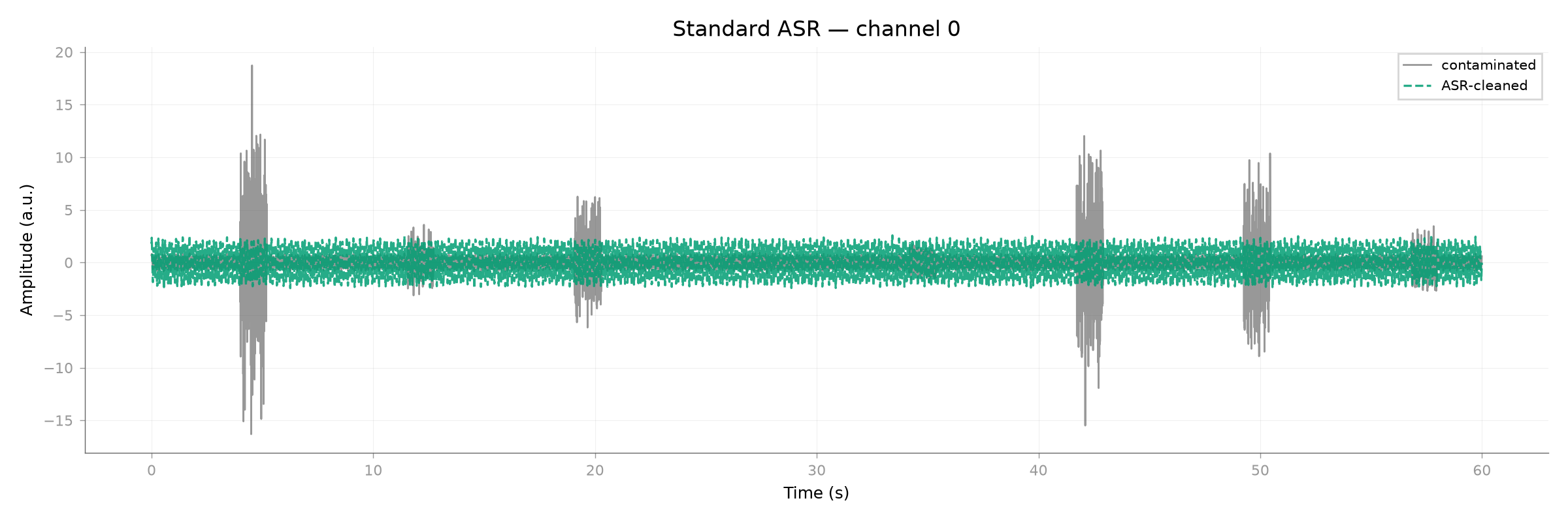
plot_signal_overlay is the generic before/after trace viewer; ASR no longer ships its own overlay wrapper.

asr = ASR(sfreq=sfreq, cutoff=20.0, picks=None, verbose=False)
cleaned = np.asarray(asr.fit_transform(contaminated))

plot_signal_overlay(
    contaminated,
    cleaned,
    t,
    pick=0,
    before_label="contaminated",
    after_label="ASR-cleaned",
    x_label="Time (s)",
    y_label="Amplitude (a.u.)",
    title="Standard ASR — channel 0",
    show=False,
)

<Figure size 2400x800 with 1 Axes>

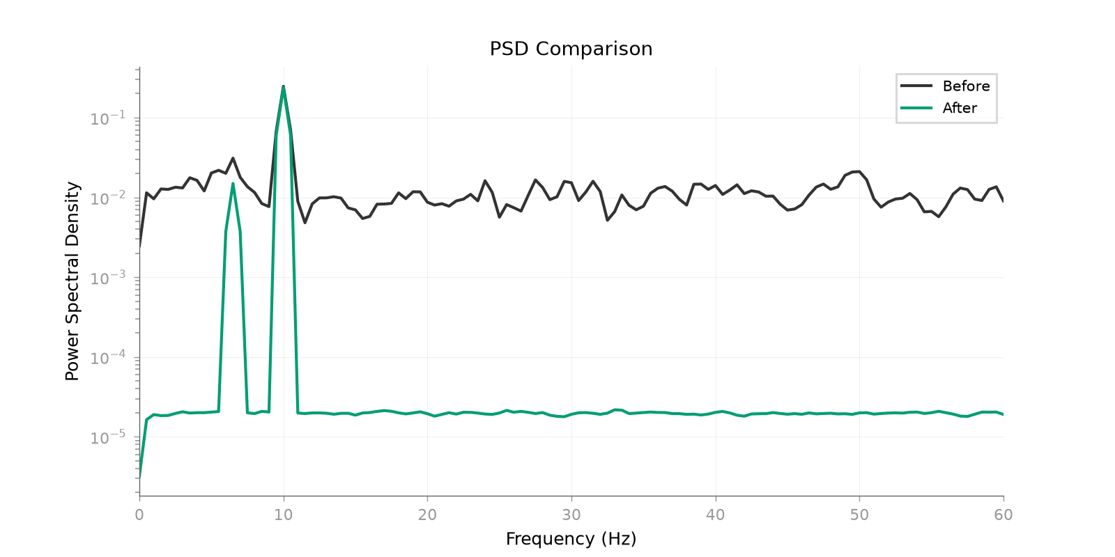
PSD before/after (generic helper)

plot_psd_comparison(contaminated, cleaned, sfreq=sfreq, fmax=60.0, show=False)

<Figure size 1600x800 with 1 Axes>

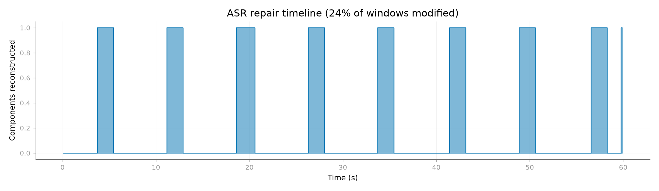
Repair timeline (ASR-specific)

Which windows were reconstructed, and how many components each lost.

plot_asr_repair_timeline(asr, show=False)

(<Figure size 2200x640 with 1 Axes>, <Axes: title={'center': 'ASR repair timeline (24% of windows modified)'}, xlabel='Time (s)', ylabel='Components reconstructed'>)

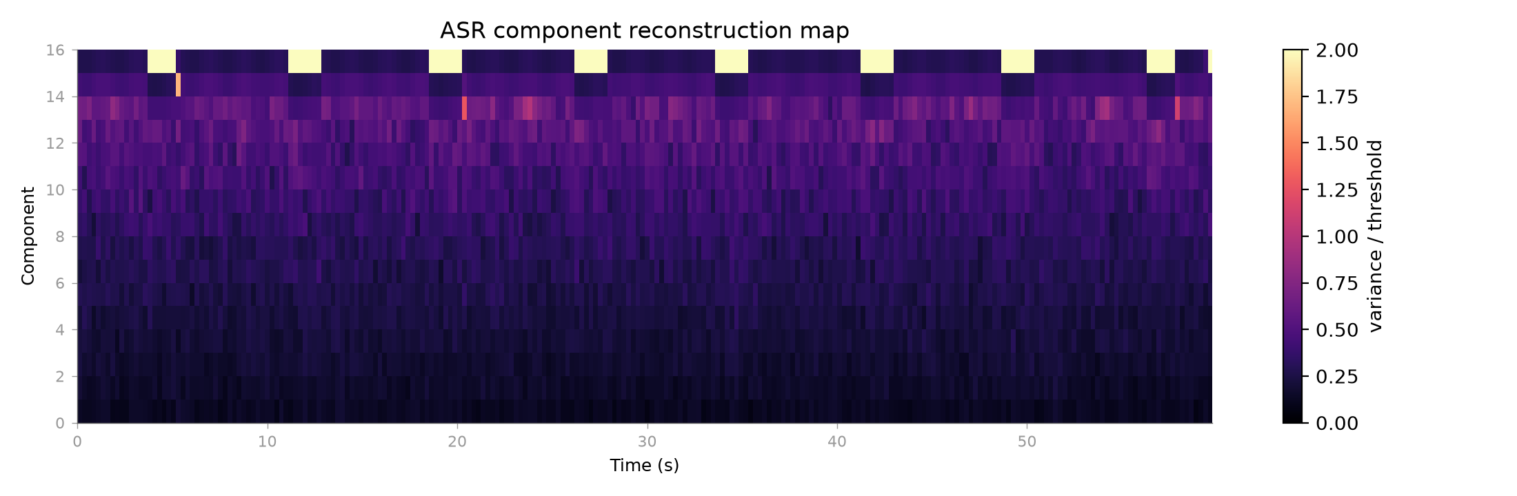
Component-reconstruction map (ASR-specific)

A window x component heatmap of the per-window principal-subspace rejection.

plot_asr_component_reconstruction(asr, show=False)

(<Figure size 2200x720 with 2 Axes>, <Axes: title={'center': 'ASR component reconstruction map'}, xlabel='Time (s)', ylabel='Component'>)

Calibration / reference fraction across variants (ASR-specific)

JugglerASR selects calibration samples point-by-point, which survives heavy contamination where the standard clean-windows criterion would struggle.

juggler = JugglerASR(
    sfreq=sfreq, cutoff=20.0, strategy="gev", picks=None, verbose=False
)
juggler.fit_transform(contaminated)
print(
    "Juggler GEV reference fraction: "
    f"{juggler.calibration_info_['reference_selected_fraction'] * 100:.1f}%"
)

plot_asr_calibration_fraction(
    [asr, juggler],
    labels=["standard", "juggler-gev"],
    title="Calibration fraction by variant",
    show=False,
)

plt.show()

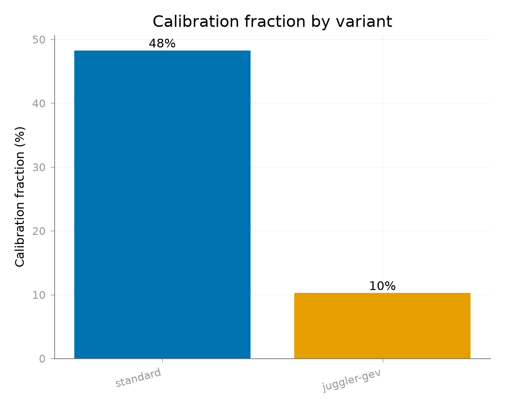
Juggler GEV reference fraction: 10.3%