BSS-CCA algorithm properties

A deterministic, synthetic demonstration of what BSS-CCA does and where it breaks. This is not a replication of any published experiment — every signal here is simulated, and the numbers depend on the simulation. For the paper-oriented experiments see scripts/replicate_declercq_paper.py.

Four properties are shown:

1. how the error depends on how many components you remove;

2. that keeping every component is exactly a no-op, including on rank-deficient data;

3. that the correlation spectrum of realistic broadband data is compressed, so a high fixed threshold is not a safe operating point;

4. that near-Nyquist energy inverts the correlation ordering unless the data is band-limited first.

import matplotlib.pyplot as plt
import numpy as np

from mne_denoise.bss_cca import compute_bss_cca
from mne_denoise.viz import themed_figure

sfreq = 250.0
n_channels, n_times = 21, int(250.0 * 10)
rng = np.random.default_rng(11)
times = np.arange(n_times) / sfreq

brain = np.vstack(
    [
        np.sin(2 * np.pi * 2.0 * times),
        np.sin(2 * np.pi * 10.0 * times + 0.4),
        np.sin(2 * np.pi * 21.0 * times + 1.1),
    ]
)
muscle = rng.standard_normal((3, n_times))
clean = rng.standard_normal((n_channels, 3)) @ brain
observed = clean + 0.8 * (rng.standard_normal((n_channels, 3)) @ muscle)
clean_centered = clean - clean.mean(axis=1, keepdims=True)


def relative_error(estimate):
    """Relative RMS error against the known clean signal."""
    return float(
        np.linalg.norm(estimate - clean_centered) / np.linalg.norm(clean_centered)
    )

1. Error as a function of how many components are removed

Three sources generated the muscle activity, and the error bottoms out at three. Removing more starts eating the neural signal.

# The sweep can only go as far as the number of components the data supports.
_, base_info = compute_bss_cca(observed, n_remove=0)
counts = np.arange(0, base_info["input_rank"] + 1)
errors = [
    relative_error(compute_bss_cca(observed, n_remove=int(k), preserve_mean=False)[0])
    for k in counts
]
for count, error in zip(counts, errors, strict=True):
    print(f"n_remove={count}: relative error {error:.4f}")

fig, ax = themed_figure(figsize=(6.0, 3.6))
ax.plot(counts, errors, marker="o")
ax.axvline(3, linestyle="--", linewidth=1, label="true number of muscle sources")
ax.set_xlabel("Components removed")
ax.set_ylabel("Relative error")
ax.set_title("Error versus components removed (synthetic)")
ax.legend()
fig.tight_layout()

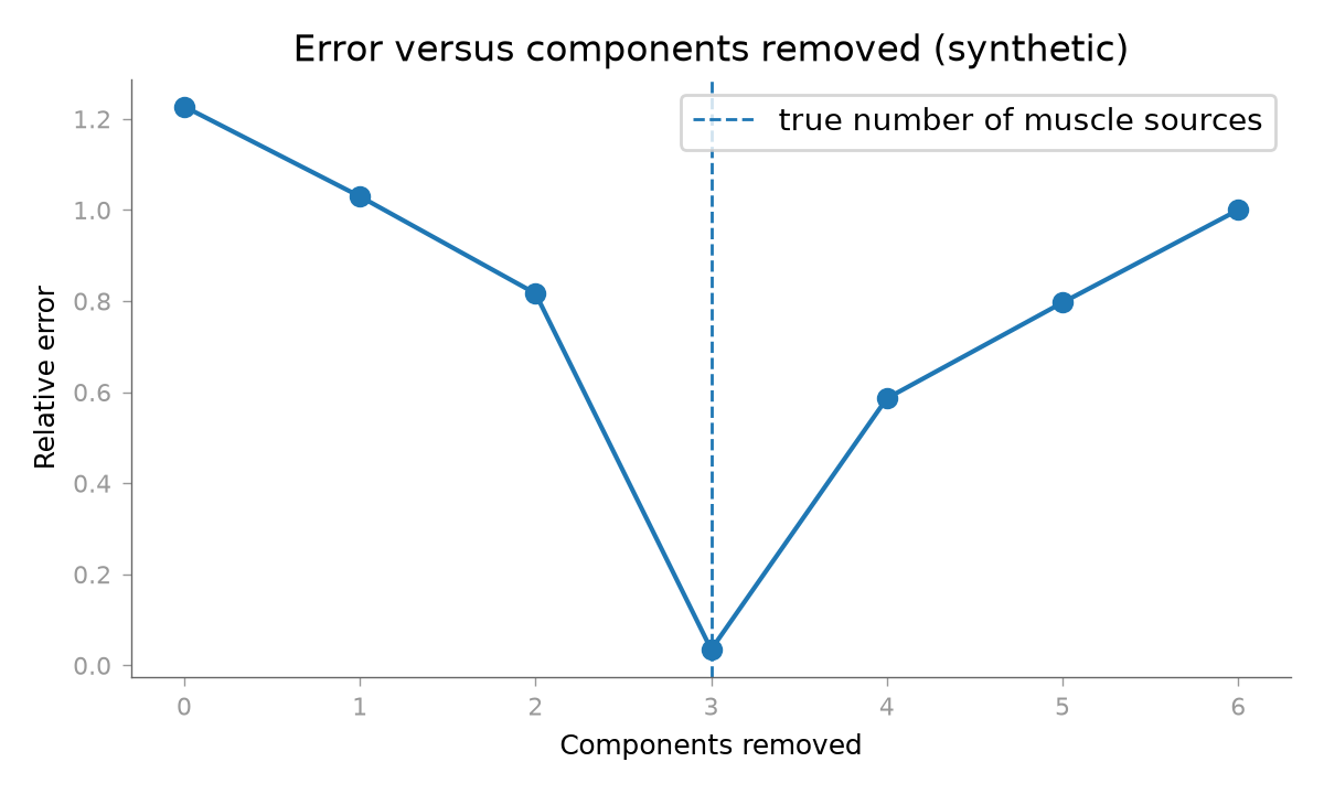
n_remove=0: relative error 1.2272
n_remove=1: relative error 1.0298
n_remove=2: relative error 0.8167
n_remove=3: relative error 0.0348
n_remove=4: relative error 0.5863
n_remove=5: relative error 0.7967
n_remove=6: relative error 1.0000

2. Keeping everything is exactly the identity

This has to hold for rank-deficient data too. Average referencing, channel interpolation, and duplicated channels all reduce the rank, and an implementation that back-projects by inverting the canonical filters silently destroys whole channels in exactly these cases.

# Start from a full-rank recording so each manipulation removes a known amount
# of rank, and the reported ranks differ.
full_rank = rng.standard_normal((12, n_times))
average_referenced = full_rank - full_rank.mean(axis=0, keepdims=True)
duplicated = full_rank.copy()
duplicated[-1] = duplicated[0]
flat = full_rank.copy()
flat[5] = 3.0

for label, data in (
    ("full rank", full_rank),
    ("average reference", average_referenced),
    ("duplicated channel", duplicated),
    ("flat channel", flat),
):
    identity, info = compute_bss_cca(data, n_remove=0, preserve_mean=True)
    residual = np.abs(identity - data).max()
    print(
        f"{label:20s} rank={info['input_rank']:3d} of {data.shape[0]}  "
        f"max deviation {residual:.2e}"
    )

full rank            rank= 12 of 12  max deviation 6.22e-15
average reference    rank= 11 of 12  max deviation 4.55e-15
duplicated channel   rank= 11 of 12  max deviation 4.33e-15
flat channel         rank= 11 of 12  max deviation 5.55e-15

3. Realistic data has a compressed correlation spectrum

The narrow-band sources above separate cleanly. Broadband neural background does not: every correlation lands in a narrow range, and a high fixed threshold would reject the entire recording.

freqs = np.fft.rfftfreq(n_times, 1.0 / sfreq)


def band_limited(n_sources, fmin, fmax):
    """Random sources restricted to a frequency band."""
    out = np.zeros((n_sources, n_times))
    for index in range(n_sources):
        spectrum = rng.standard_normal(freqs.size) + 1j * rng.standard_normal(
            freqs.size
        )
        spectrum[(freqs < fmin) | (freqs > fmax)] = 0.0
        out[index] = np.fft.irfft(spectrum, n=n_times)
    return out / np.linalg.norm(out)


broadband_brain = band_limited(6, 1.0, 45.0)
broadband_muscle = band_limited(3, 30.0, sfreq / 2)
realistic = rng.standard_normal((n_channels, 6)) @ broadband_brain
realistic = realistic + 1.2 * (rng.standard_normal((n_channels, 3)) @ broadband_muscle)

_, narrow_info = compute_bss_cca(observed, n_remove=3)
_, wide_info = compute_bss_cca(realistic, n_remove=3)
print(f"narrow-band correlations: {np.round(narrow_info['correlations'][:6], 3)}")
print(f"broadband correlations:   {np.round(wide_info['correlations'][:6], 3)}")
print(f"broadband maximum:        {wide_info['correlations'].max():.3f}")

fig, ax = themed_figure(figsize=(6.0, 3.6))
ax.plot(narrow_info["correlations"], marker="o", label="narrow-band sources")
ax.plot(wide_info["correlations"], marker="s", label="broadband sources")
ax.set_xlabel("Component")
ax.set_ylabel("Canonical correlation")
ax.set_title("Correlation spectrum depends on the signal regime (synthetic)")
ax.legend()
fig.tight_layout()

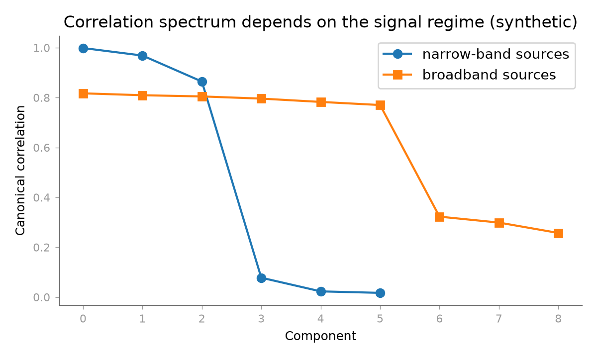
narrow-band correlations: [0.999 0.969 0.864 0.078 0.023 0.017]
broadband correlations:   [0.817 0.809 0.805 0.796 0.783 0.77 ]
broadband maximum:        0.817

4. Near-Nyquist energy inverts the ordering

Canonical correlations come from singular values and are never negative, so a component oscillating at the Nyquist frequency is anti-correlated at lag 1 yet receives a correlation near 1. Band-limit before decomposing, as both source papers do, and check autocorrelations for negative entries.

aliased_sources = np.zeros((6, n_times))
aliased_sources[0] = (-1.0) ** np.arange(n_times)
aliased_sources[1:] = rng.standard_normal((5, n_times))
aliased = rng.standard_normal((6, 6)) @ aliased_sources

_, aliased_info = compute_bss_cca(aliased, n_remove=1)
worst = int(np.argmin(aliased_info["autocorrelations"]))
print(f"correlations:    {np.round(aliased_info['correlations'], 3)}")
print(f"autocorrelations:{np.round(aliased_info['autocorrelations'], 3)}")
print(
    f"component {worst} ranks at correlation "
    f"{aliased_info['correlations'][worst]:.3f} but is anti-correlated "
    f"({aliased_info['autocorrelations'][worst]:.3f})"
)

fig, ax = themed_figure(figsize=(6.0, 3.6))
index = np.arange(aliased_info["correlations"].size)
ax.bar(index - 0.2, aliased_info["correlations"], width=0.4, label="canonical rho")
ax.bar(
    index + 0.2,
    aliased_info["autocorrelations"],
    width=0.4,
    label="signed autocorrelation",
)
ax.axhline(0.0, linewidth=1)
ax.set_xlabel("Component")
ax.set_ylabel("Value")
ax.set_title("Unfiltered data: rho hides the sign (synthetic)")
ax.legend()
fig.tight_layout()

plt.show()

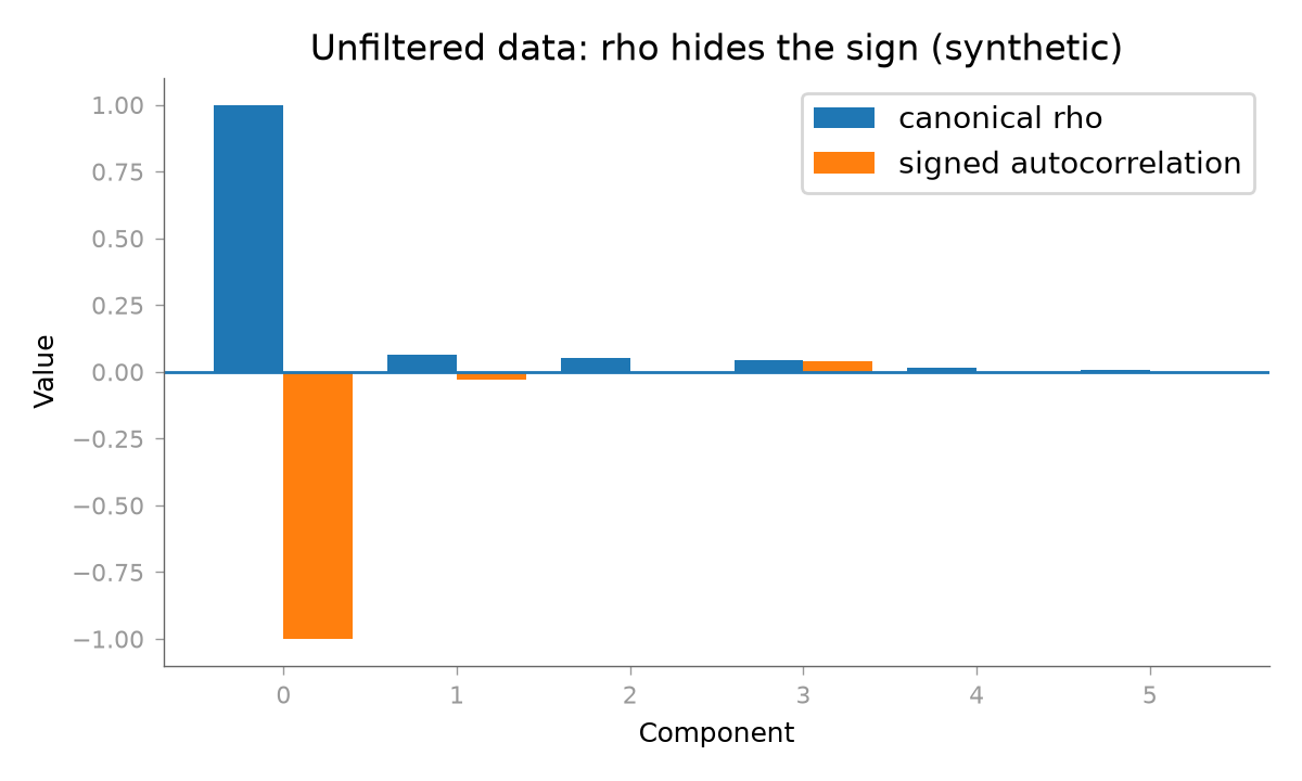
correlations:    [1.    0.065 0.053 0.044 0.017 0.006]
autocorrelations:[-1.    -0.031 -0.004  0.039 -0.002  0.001]
component 0 ranks at correlation 1.000 but is anti-correlated (-1.000)