Quantifying Dataset Noise with RMS Statistics

This example demonstrates how to use ASR’s robust mathematical estimators independently of the full ASR pipeline to quantify the baseline noisiness of a dataset.

We use the fit_rms_distribution function. This function takes a distribution of window-RMS values, ignores the extreme artifact tails, and fits a Generalized Gaussian curve to the clean data. This allows researchers to calculate robust location (mu) and scale (sigma) statistics to standardize or compare subjects.

Imports

import matplotlib.pyplot as plt
import numpy as np

from mne_denoise.asr import fit_rms_distribution

Part 1: Synthetic Data

Let’s generate a synthetic distribution of RMS values. Real EEG/MEG RMS values often follow a Generalized Gaussian distribution, but are heavily contaminated by large, positive “tails” caused by artifacts like eye blinks or movement.

rng = np.random.default_rng(42)

# Simulate clean brain RMS data (mean=10.0, std=2.0)
clean_rms = np.abs(rng.normal(loc=10.0, scale=2.0, size=5000))

# Simulate massive artifact RMS data (mean=30.0, std=10.0)
artifact_rms = np.abs(rng.normal(loc=30.0, scale=10.0, size=500))

# Combine them into a single contaminated dataset
contaminated_rms = np.concatenate([clean_rms, artifact_rms])
np.random.shuffle(contaminated_rms)

print(f"Total simulated windows: {len(contaminated_rms)}")

Total simulated windows: 5500

Fitting the Distribution

If we used standard mean and standard deviation on this dataset, the massive artifacts would severely distort the results. Instead, we use fit_rms_distribution to ignore the artifact tails and fit the true clean core.

standard_mean = np.mean(contaminated_rms)
standard_std = np.std(contaminated_rms)

# We set return_info=True to get the exact fitted shape parameter (beta)
mu, sigma, info = fit_rms_distribution(contaminated_rms, return_info=True)

print("\n--- Standard Statistics ---")
print(f"Mean: {standard_mean:.2f}")
print(f"Std:  {standard_std:.2f}")

print("\n--- Robust RMS Statistics ---")
print(f"Mu (Clean Center): {mu:.2f}")
print(f"Sigma (Clean Spread): {sigma:.2f}")
print(f"Beta (Curve Shape): {info['beta']:.2f}")

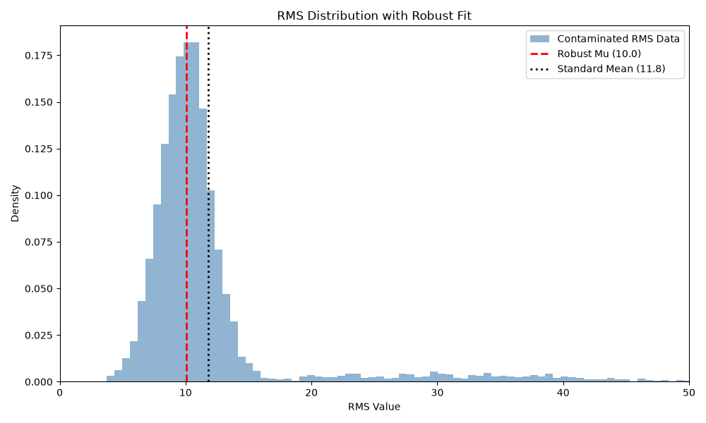
# Notice how `mu` perfectly locked onto the true clean mean (10.0), while
# the standard mean was artificially dragged up by the artifacts.

--- Standard Statistics ---
Mean: 11.81
Std:  6.84

--- Robust RMS Statistics ---
Mu (Clean Center): 10.04
Sigma (Clean Spread): 2.01
Beta (Curve Shape): 2.00

Visualizing the Fit

We can visualize the distribution to see exactly what the algorithm did. The algorithm found the main peak and ignored the long right tail.

fig, ax = plt.subplots(figsize=(10, 6))

# Plot the raw histogram
counts, bins, _ = ax.hist(
    contaminated_rms,
    bins=100,
    density=True,
    alpha=0.6,
    color="steelblue",
    label="Contaminated RMS Data",
)

# Plot the robust center
ax.axvline(mu, color="red", linestyle="--", linewidth=2, label=f"Robust Mu ({mu:.1f})")
ax.axvline(
    standard_mean,
    color="black",
    linestyle=":",
    linewidth=2,
    label=f"Standard Mean ({standard_mean:.1f})",
)

ax.set_title("RMS Distribution with Robust Fit")
ax.set_xlabel("RMS Value")
ax.set_ylabel("Density")
ax.set_xlim(0, 50)
ax.legend()
plt.tight_layout()
plt.show(block=False)

Part 2: Real Data

In practice, you would calculate these RMS values yourself directly from your continuous data by sliding a window across it and calculating the RMS of the variance for each window.

This allows you to quantify “how noisy is this subject compared to the cohort?” or to Z-score your data robustly prior to downstream machine learning.