Note
Click here to download the full example code
The Evoked data structure: evoked/averaged data#
This tutorial covers the basics of creating and working with evoked
data. It introduces the Evoked data structure in detail,
including how to load, query, subselect, export, and plot data from an
Evoked object. For info on creating an Evoked
object from (possibly simulated) data in a NumPy array, see Creating MNE-Python data structures from scratch.
As usual we’ll start by importing the modules we need:
import os
import mne
Creating Evoked objects from Epochs#
Evoked objects typically store an EEG or MEG signal that has
been averaged over multiple epochs, which is a common technique for
estimating stimulus-evoked activity. The data in an Evoked
object are stored in an array of shape
(n_channels, n_times) (in contrast to an Epochs object,
which stores data of shape (n_epochs, n_channels, n_times)). Thus to
create an Evoked object, we’ll start by epoching some raw data,
and then averaging together all the epochs from one condition:
sample_data_folder = mne.datasets.sample.data_path()
sample_data_raw_file = os.path.join(sample_data_folder, 'MEG', 'sample',
                                    'sample_audvis_raw.fif')
raw = mne.io.read_raw_fif(sample_data_raw_file, verbose=False)
events = mne.find_events(raw, stim_channel='STI 014')
# we'll skip the "face" and "buttonpress" conditions, to save memory:
event_dict = {'auditory/left': 1, 'auditory/right': 2, 'visual/left': 3,
              'visual/right': 4}
epochs = mne.Epochs(raw, events, tmin=-0.3, tmax=0.7, event_id=event_dict,
                    preload=True)
evoked = epochs['auditory/left'].average()

del raw  # reduce memory usage
320 events found
Event IDs: [ 1  2  3  4  5 32]
Not setting metadata
289 matching events found
Setting baseline interval to [-0.2996928197375818, 0.0] sec
Applying baseline correction (mode: mean)
Created an SSP operator (subspace dimension = 3)
3 projection items activated
Loading data for 289 events and 601 original time points ...
0 bad epochs dropped
You may have noticed that MNE informed us that “baseline correction” has been
applied. This happened automatically by during creation of the
Epochs object, but may also be initiated (or disabled!) manually:
We will discuss this in more detail later.
The information about the baseline period of Epochs is transferred to
derived Evoked objects to maintain provenance as you process your
data:
print(f'Epochs baseline: {epochs.baseline}')
print(f'Evoked baseline: {evoked.baseline}')
Epochs baseline: (-0.2996928197375818, 0.0)
Evoked baseline: (-0.2996928197375818, 0.0)
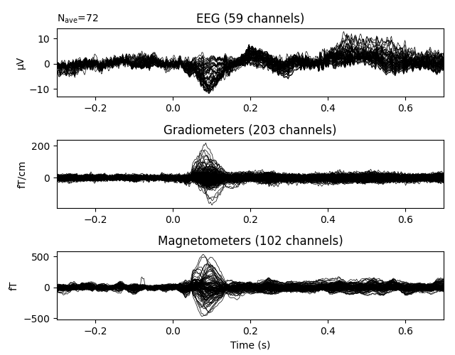
Basic visualization of Evoked objects#
We can visualize the average evoked response for left-auditory stimuli using
the plot() method, which yields a butterfly plot of each
channel type:
Like the plot() methods for Raw and
Epochs objects,
evoked.plot() has many parameters for customizing
the plot output, such as color-coding channel traces by scalp location, or
plotting the global field power alongside the channel traces.
See Visualizing Evoked data for more information about visualizing
Evoked objects.
Subselecting Evoked data#
Unlike Raw and Epochs objects,
Evoked objects do not support selection by square-bracket
indexing. Instead, data can be subselected by indexing the
data attribute:
print(evoked.data[:2, :3]) # first 2 channels, first 3 timepoints
[[ 5.72160572e-13  3.57859354e-13  3.98040833e-13]
 [-2.75128428e-13 -3.15309907e-13 -5.83186429e-13]]
To select based on time in seconds, the time_as_index()
method can be useful, although beware that depending on the sampling
frequency, the number of samples in a span of given duration may not always
be the same (see the Time, sample number, and sample index section of the
tutorial about Raw data for details).
Selecting, dropping, and reordering channels#
By default, when creating Evoked data from an
Epochs object, only the “data” channels will be retained:
eog, ecg, stim, and misc channel types will be dropped. You
can control which channel types are retained via the picks parameter of
epochs.average(), by passing 'all' to
retain all channels, or by passing a list of integers, channel names, or
channel types. See the documentation of average() for
details.
If you’ve already created the Evoked object, you can use the
pick(), pick_channels(),
pick_types(), and drop_channels() methods
to modify which channels are included in an Evoked object.
You can also use reorder_channels() for this purpose; any
channel names not provided to reorder_channels() will be
dropped. Note that channel selection methods modify the object in-place, so
in interactive/exploratory sessions you may want to create a
copy() first.
evoked_eeg = evoked.copy().pick_types(meg=False, eeg=True)
print(evoked_eeg.ch_names)

new_order = ['EEG 002', 'MEG 2521', 'EEG 003']
evoked_subset = evoked.copy().reorder_channels(new_order)
print(evoked_subset.ch_names)
Removing projector <Projection | PCA-v1, active : True, n_channels : 102>
Removing projector <Projection | PCA-v2, active : True, n_channels : 102>
Removing projector <Projection | PCA-v3, active : True, n_channels : 102>
['EEG 001', 'EEG 002', 'EEG 003', 'EEG 004', 'EEG 005', 'EEG 006', 'EEG 007', 'EEG 008', 'EEG 009', 'EEG 010', 'EEG 011', 'EEG 012', 'EEG 013', 'EEG 014', 'EEG 015', 'EEG 016', 'EEG 017', 'EEG 018', 'EEG 019', 'EEG 020', 'EEG 021', 'EEG 022', 'EEG 023', 'EEG 024', 'EEG 025', 'EEG 026', 'EEG 027', 'EEG 028', 'EEG 029', 'EEG 030', 'EEG 031', 'EEG 032', 'EEG 033', 'EEG 034', 'EEG 035', 'EEG 036', 'EEG 037', 'EEG 038', 'EEG 039', 'EEG 040', 'EEG 041', 'EEG 042', 'EEG 043', 'EEG 044', 'EEG 045', 'EEG 046', 'EEG 047', 'EEG 048', 'EEG 049', 'EEG 050', 'EEG 051', 'EEG 052', 'EEG 054', 'EEG 055', 'EEG 056', 'EEG 057', 'EEG 058', 'EEG 059', 'EEG 060']
['EEG 002', 'MEG 2521', 'EEG 003']
Similarities among the core data structures#
Evoked objects have many similarities with Raw
and Epochs objects, including:
They can be loaded from and saved to disk in
.fifformat, and their data can be exported to aNumPy array(but through thedataattribute, not through aget_data()method).Pandas DataFrameexport is also available through theto_data_frame()method.You can change the name or type of a channel using
evoked.rename_channels()orevoked.set_channel_types(). Both methods takedictionarieswhere the keys are existing channel names, and the values are the new name (or type) for that channel. Existing channels that are not in the dictionary will be unchanged.SSP projector manipulation is possible through
add_proj(),del_proj(), andplot_projs_topomap()methods, and theprojattribute. See Repairing artifacts with SSP for more information on SSP.Like
RawandEpochsobjects,Evokedobjects havecopy(),crop(),time_as_index(),filter(), andresample()methods.Like
RawandEpochsobjects,Evokedobjects haveevoked.times,evoked.ch_names, andinfoattributes.
Loading and saving Evoked data#
Single Evoked objects can be saved to disk with the
evoked.save() method. One difference between
Evoked objects and the other data structures is that multiple
Evoked objects can be saved into a single .fif file, using
mne.write_evokeds(). The example data
includes just such a .fif file: the data have already been epoched and
averaged, and the file contains separate Evoked objects for
each experimental condition:
sample_data_evk_file = os.path.join(sample_data_folder, 'MEG', 'sample',
                                    'sample_audvis-ave.fif')
evokeds_list = mne.read_evokeds(sample_data_evk_file, verbose=False)
print(evokeds_list)
print(type(evokeds_list))
[<Evoked | 'Left Auditory' (average, N=55), -0.1998 – 0.49949 sec, baseline off, 376 ch, ~4.5 MB>, <Evoked | 'Right Auditory' (average, N=61), -0.1998 – 0.49949 sec, baseline off, 376 ch, ~4.5 MB>, <Evoked | 'Left visual' (average, N=67), -0.1998 – 0.49949 sec, baseline off, 376 ch, ~4.5 MB>, <Evoked | 'Right visual' (average, N=58), -0.1998 – 0.49949 sec, baseline off, 376 ch, ~4.5 MB>]
<class 'list'>
Notice that mne.read_evokeds() returned a list of
Evoked objects, and each one has an evoked.comment
attribute describing the experimental condition that was averaged to
generate the estimate:
for evok in evokeds_list:
    print(evok.comment)
Left Auditory
Right Auditory
Left visual
Right visual
If you want to load only some of the conditions present in a .fif file,
read_evokeds() has a condition parameter, which takes either a
string (matched against the comment attribute of the evoked objects on disk),
or an integer selecting the Evoked object based on the order
it’s stored in the file. Passing lists of integers or strings is also
possible. If only one object is selected, the Evoked object
will be returned directly (rather than a length-one list containing it):
right_vis = mne.read_evokeds(sample_data_evk_file, condition='Right visual')
print(right_vis)
print(type(right_vis))
Reading /home/circleci/mne_data/MNE-sample-data/MEG/sample/sample_audvis-ave.fif ...
    Read a total of 4 projection items:
        PCA-v1 (1 x 10²) active
        PCA-v2 (1 x 10²) active
        PCA-v3 (1 x 10²) active
        Average EEG reference (1 x 60) active
    Found the data of interest:
        t =    -199.80 ...     499.49 ms (Right visual)
        0 CTF compensation matrices available
        nave = 58 - aspect type = 100
Projections have already been applied. Setting proj attribute to True.
No baseline correction applied
<Evoked | 'Right visual' (average, N=58), -0.1998 – 0.49949 sec, baseline off, 376 ch, ~4.5 MB>
<class 'mne.evoked.Evoked'>
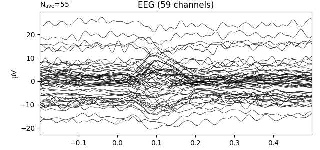
Above, when we created an Evoked object by averaging epochs,
baseline correction was applied by default when we extracted epochs from the
Raw object (the default baseline period is (None, 0),
which assured zero mean for times before the stimulus event). In contrast, if
we plot the first Evoked object in the list that was loaded
from disk, we’ll see that the data have not been baseline-corrected:
evokeds_list[0].plot(picks='eeg')
This can be remedied by either passing a baseline parameter to
mne.read_evokeds(), or by applying baseline correction after loading,
as shown here:
# Original baseline (none set).
print(f'Baseline after loading: {evokeds_list[0].baseline}')
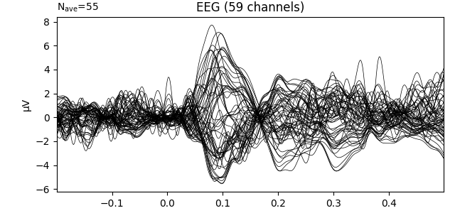
# Apply a custom baseline correction.
evokeds_list[0].apply_baseline((None, 0))
print(f'Baseline after calling apply_baseline(): {evokeds_list[0].baseline}')
# Visualize the evoked response.
evokeds_list[0].plot(picks='eeg')
Baseline after loading: None
Applying baseline correction (mode: mean)
Baseline after calling apply_baseline(): (-0.19979521315838786, 0.0)
Notice that apply_baseline() operated in-place. Similarly,
Evoked objects may have been saved to disk with or without
projectors applied; you can pass proj=True to the
read_evokeds() function, or use the apply_proj()
method after loading.
Combining Evoked objects#
One way to pool data across multiple conditions when estimating evoked
responses is to do so prior to averaging (recall that MNE-Python can select
based on partial matching of /-separated epoch labels; see
Subselecting epochs for more info):
left_right_aud = epochs['auditory'].average()
print(left_right_aud)
<Evoked | '0.50 × auditory/left + 0.50 × auditory/right' (average, N=145), -0.29969 – 0.69928 sec, baseline -0.299693 – 0 sec, 366 ch, ~5.0 MB>
This approach will weight each epoch equally and create a single
Evoked object. Notice that the printed representation includes
(average, N=145), indicating that the Evoked object was
created by averaging across 145 epochs. In this case, the event types were
fairly close in number:
[72, 73]
However, this may not always be the case; if for statistical reasons it is
important to average the same number of epochs from different conditions,
you can use equalize_event_counts() prior to averaging.
Another approach to pooling across conditions is to create separate
Evoked objects for each condition, and combine them afterward.
This can be accomplished by the function mne.combine_evoked(), which
computes a weighted sum of the Evoked objects given to it. The
weights can be manually specified as a list or array of float values, or can
be specified using the keyword 'equal' (weight each Evoked object
by \(\frac{1}{N}\), where \(N\) is the number of Evoked
objects given) or the keyword 'nave' (weight each Evoked object
proportional to the number of epochs averaged together to create it):
left_right_aud = mne.combine_evoked([left_aud, right_aud], weights='nave')
assert left_right_aud.nave == left_aud.nave + right_aud.nave
Note that the nave attribute of the resulting Evoked object will
reflect the effective number of averages, and depends on both the nave
attributes of the contributing Evoked objects and the weights at
which they are combined. Keeping track of effective nave is important for
inverse imaging, because nave is used to scale the noise covariance
estimate (which in turn affects the magnitude of estimated source activity).
See The minimum-norm current estimates for more information (especially the
Whitening and scaling section). Note that mne.grand_average does
not adjust nave to reflect effective number of averaged epochs; rather
it simply sets nave to the number of evokeds that were averaged
together. For this reason, it is best to use mne.combine_evoked rather than
mne.grand_average if you intend to perform inverse imaging on the resulting
Evoked object.
Other uses of Evoked objects#
Although the most common use of Evoked objects is to store
averages of epoched data, there are a couple other uses worth noting here.
First, the method epochs.standard_error()
will create an Evoked object (just like
epochs.average() does), but the data in the
Evoked object will be the standard error across epochs instead
of the average. To indicate this difference, Evoked objects
have a kind attribute that takes values 'average' or
'standard error' as appropriate.
Another use of Evoked objects is to represent a single trial
or epoch of data, usually when looping through epochs. This can be easily
accomplished with the epochs.iter_evoked()
method, and can be useful for applications where you want to do something
that is only possible for Evoked objects. For example, here
we use the get_peak() method (which isn’t available for
Epochs objects) to get the peak response in each trial:
for ix, trial in enumerate(epochs[:3].iter_evoked()):
    channel, latency, value = trial.get_peak(ch_type='eeg',
                                             return_amplitude=True)
    latency = int(round(latency * 1e3))  # convert to milliseconds
    value = int(round(value * 1e6))      # convert to µV
    print('Trial {}: peak of {} µV at {} ms in channel {}'
          .format(ix, value, latency, channel))
Trial 0: peak of 159 µV at 35 ms in channel EEG 003
Trial 1: peak of -45 µV at 569 ms in channel EEG 005
Trial 2: peak of -46 µV at 648 ms in channel EEG 015
Total running time of the script: ( 0 minutes 14.746 seconds)
Estimated memory usage: 757 MB