Note
Click here to download the full example code
Brainstorm Elekta phantom dataset tutorial#
Here we compute the evoked from raw for the Brainstorm Elekta phantom tutorial dataset. For comparison, see 1 and the original Brainstorm tutorial.
# Authors: Eric Larson <larson.eric.d@gmail.com>
#
# License: BSD-3-Clause
import os.path as op
import numpy as np
import matplotlib.pyplot as plt

import mne
from mne import find_events, fit_dipole
from mne.datasets import fetch_phantom
from mne.datasets.brainstorm import bst_phantom_elekta
from mne.io import read_raw_fif

print(__doc__)
The data were collected with an Elekta Neuromag VectorView system at 1000 Hz
and low-pass filtered at 330 Hz. Here the medium-amplitude (200 nAm) data
are read to construct instances of mne.io.Raw.
data_path = bst_phantom_elekta.data_path(verbose=True)

raw_fname = op.join(data_path, 'kojak_all_200nAm_pp_no_chpi_no_ms_raw.fif')
raw = read_raw_fif(raw_fname)
Opening raw data file /home/circleci/mne_data/MNE-brainstorm-data/bst_phantom_elekta/kojak_all_200nAm_pp_no_chpi_no_ms_raw.fif...
    Read a total of 13 projection items:
        planar-0.0-115.0-PCA-01 (1 x 306)  idle
        planar-0.0-115.0-PCA-02 (1 x 306)  idle
        planar-0.0-115.0-PCA-03 (1 x 306)  idle
        planar-0.0-115.0-PCA-04 (1 x 306)  idle
        planar-0.0-115.0-PCA-05 (1 x 306)  idle
        axial-0.0-115.0-PCA-01 (1 x 306)  idle
        axial-0.0-115.0-PCA-02 (1 x 306)  idle
        axial-0.0-115.0-PCA-03 (1 x 306)  idle
        axial-0.0-115.0-PCA-04 (1 x 306)  idle
        axial-0.0-115.0-PCA-05 (1 x 306)  idle
        axial-0.0-115.0-PCA-06 (1 x 306)  idle
        axial-0.0-115.0-PCA-07 (1 x 306)  idle
        axial-0.0-115.0-PCA-08 (1 x 306)  idle
    Range : 47000 ... 437999 =     47.000 ...   437.999 secs
Ready.
Data channel array consisted of 204 MEG planor gradiometers, 102 axial magnetometers, and 3 stimulus channels. Let’s get the events for the phantom, where each dipole (1-32) gets its own event:

645 events found
Event IDs: [   1    2    3    4    5    6    7    8    9   10   11   12   13   14
   15   16   17   18   19   20   21   22   23   24   25   26   27   28
   29   30   31   32  256  768 1792 3840 7936]
Opening raw-browser...
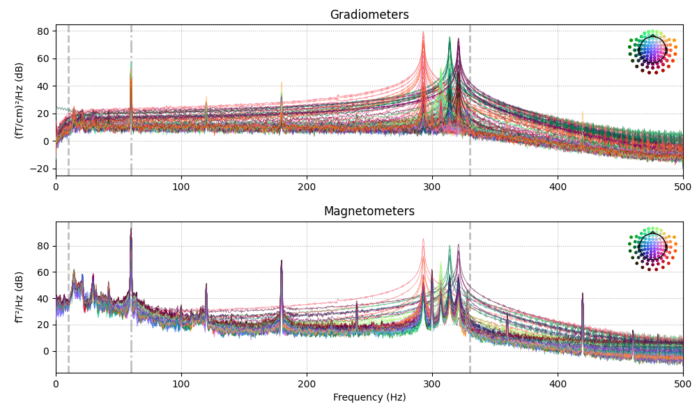
The data have strong line frequency (60 Hz and harmonics) and cHPI coil noise (five peaks around 300 Hz). Here we plot only out to 60 seconds to save memory:
raw.plot_psd(tmax=30., average=False)
Effective window size : 2.048 (s)
Effective window size : 2.048 (s)
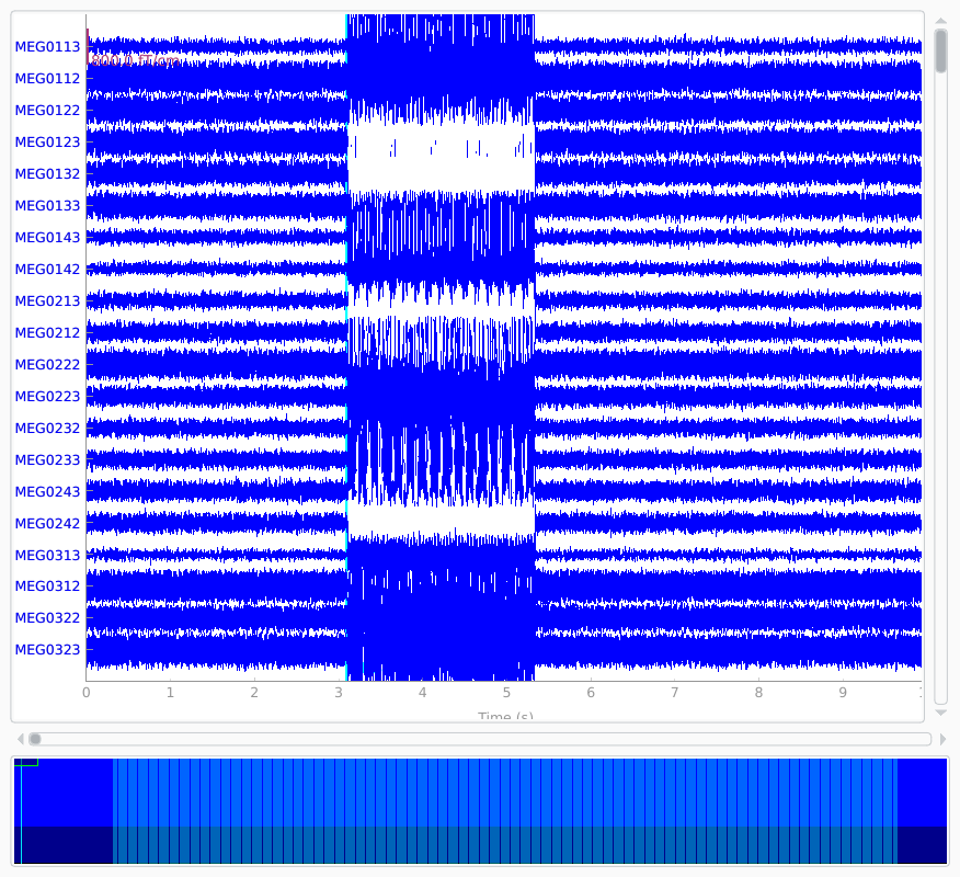
Our phantom produces sinusoidal bursts at 20 Hz:
Opening raw-browser...
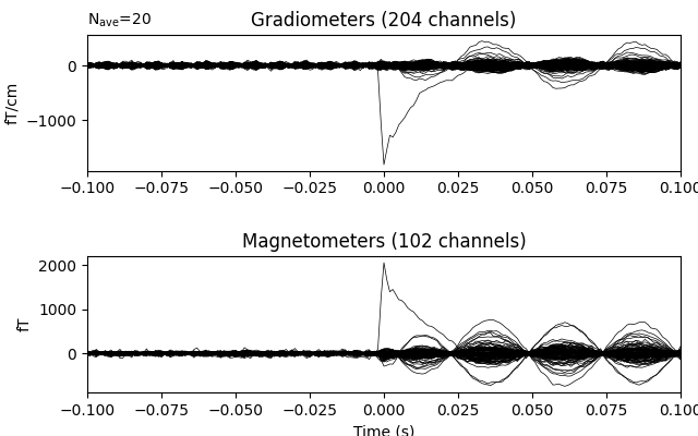
Now we epoch our data, average it, and look at the first dipole response. The first peak appears around 3 ms. Because we low-passed at 40 Hz, we can also decimate our data to save memory.
Not setting metadata
640 matching events found
Setting baseline interval to [-0.1, -0.05] sec
Applying baseline correction (mode: mean)
Created an SSP operator (subspace dimension = 13)
13 projection items activated
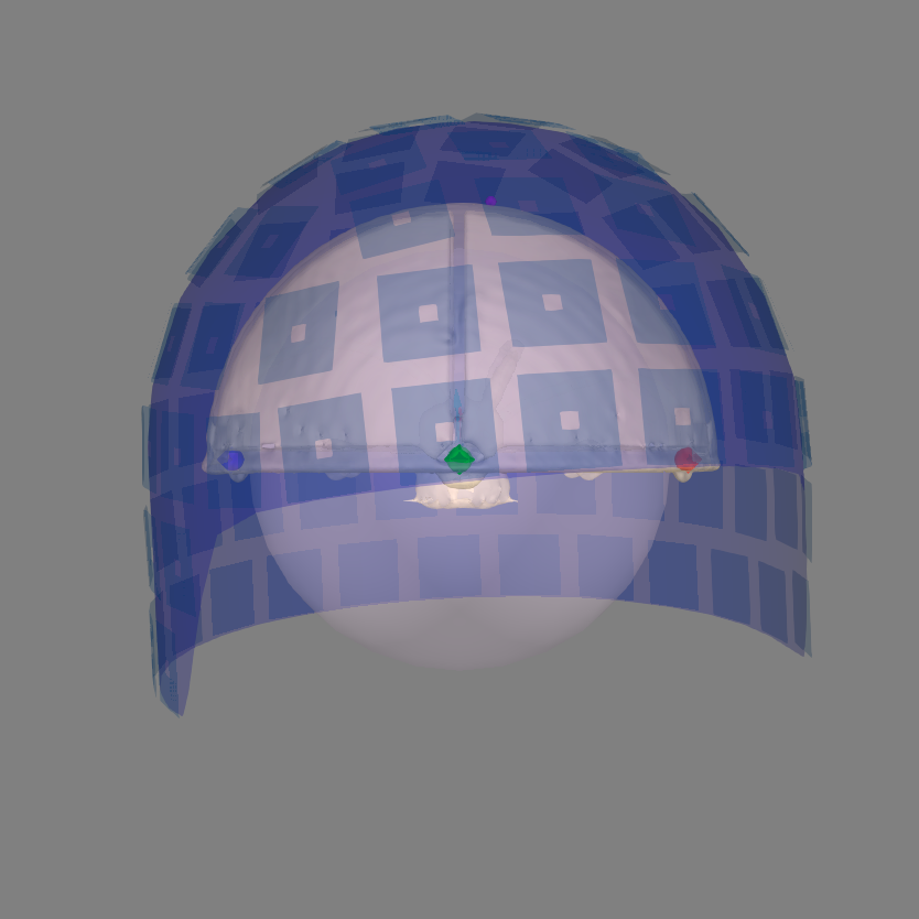
Let’s use a sphere head geometry model and let’s see the coordinate alignment and the sphere location. The phantom is properly modeled by a single-shell sphere with origin (0., 0., 0.).
Even though this is a VectorView/TRIUX phantom, we can use the Otaniemi
phantom subject as a surrogate because the “head” surface (hemisphere outer
shell) has the same geometry for both phantoms, even though the internal
dipole locations differ. The phantom_otaniemi scan was aligned to the
phantom’s head coordinate frame, so an identity trans is appropriate
here.
subjects_dir = data_path
fetch_phantom('otaniemi', subjects_dir=subjects_dir)
sphere = mne.make_sphere_model(r0=(0., 0., 0.), head_radius=0.08)
subject = 'phantom_otaniemi'
trans = mne.transforms.Transform('head', 'mri', np.eye(4))
mne.viz.plot_alignment(
    epochs.info, subject=subject, show_axes=True, bem=sphere, dig=True,
    surfaces=('head-dense', 'inner_skull'), trans=trans, mri_fiducials=True,
    subjects_dir=subjects_dir)
0 files missing from phantom_otaniemi.txt in /home/circleci/mne_data/MNE-brainstorm-data/bst_phantom_elekta

Equiv. model fitting -> RV = 0.00372821 %
mu1 = 0.943946    lambda1 = 0.139079
mu2 = 0.665521    lambda2 = 0.684839
mu3 = -0.0973038    lambda3 = -0.013548
Set up EEG sphere model with scalp radius    80.0 mm

Using lh.seghead for head surface.
Getting helmet for system 306m
Channel types:: grad: 204, mag: 102
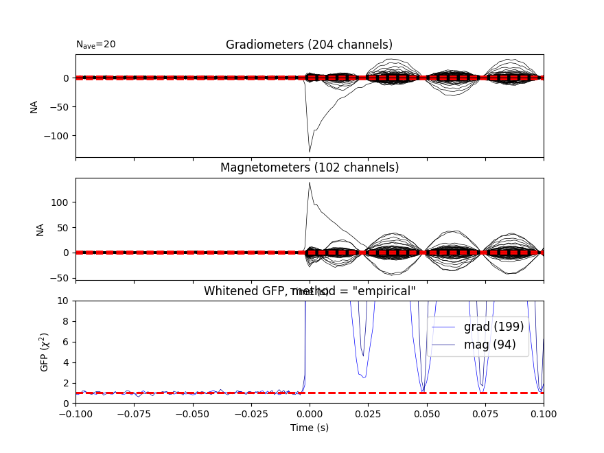
Let’s do some dipole fits. We first compute the noise covariance, then do the fits for each event_id taking the time instant that maximizes the global field power.
# here we can get away with using method='oas' for speed (faster than "shrunk")
# but in general "shrunk" is usually better
cov = mne.compute_covariance(epochs, tmax=bmax)
mne.viz.plot_evoked_white(epochs['1'].average(), cov)

data = []
t_peak = 0.036  # true for Elekta phantom
for ii in event_id:
    # Avoid the first and last trials -- can contain dipole-switching artifacts
    evoked = epochs[str(ii)][1:-1].average().crop(t_peak, t_peak)
    data.append(evoked.data[:, 0])
evoked = mne.EvokedArray(np.array(data).T, evoked.info, tmin=0.)
del epochs
dip, residual = fit_dipole(evoked, cov, sphere, n_jobs=1)
Loading data for 20 events and 201 original time points ...
0 bad epochs dropped
Loading data for 20 events and 201 original time points ...
0 bad epochs dropped
Loading data for 20 events and 201 original time points ...
0 bad epochs dropped
Loading data for 20 events and 201 original time points ...
0 bad epochs dropped
Loading data for 20 events and 201 original time points ...
0 bad epochs dropped
Loading data for 20 events and 201 original time points ...
0 bad epochs dropped
Loading data for 20 events and 201 original time points ...
0 bad epochs dropped
Loading data for 20 events and 201 original time points ...
0 bad epochs dropped
Loading data for 20 events and 201 original time points ...
0 bad epochs dropped
Loading data for 20 events and 201 original time points ...
0 bad epochs dropped
Loading data for 20 events and 201 original time points ...
0 bad epochs dropped
Loading data for 20 events and 201 original time points ...
0 bad epochs dropped
Loading data for 20 events and 201 original time points ...
0 bad epochs dropped
Loading data for 20 events and 201 original time points ...
0 bad epochs dropped
Loading data for 20 events and 201 original time points ...
0 bad epochs dropped
Loading data for 20 events and 201 original time points ...
0 bad epochs dropped
Loading data for 20 events and 201 original time points ...
0 bad epochs dropped
Loading data for 20 events and 201 original time points ...
0 bad epochs dropped
Loading data for 20 events and 201 original time points ...
0 bad epochs dropped
Loading data for 20 events and 201 original time points ...
0 bad epochs dropped
Loading data for 20 events and 201 original time points ...
0 bad epochs dropped
Loading data for 20 events and 201 original time points ...
0 bad epochs dropped
Loading data for 20 events and 201 original time points ...
0 bad epochs dropped
Loading data for 20 events and 201 original time points ...
0 bad epochs dropped
Loading data for 20 events and 201 original time points ...
0 bad epochs dropped
Loading data for 20 events and 201 original time points ...
0 bad epochs dropped
Loading data for 20 events and 201 original time points ...
0 bad epochs dropped
Loading data for 20 events and 201 original time points ...
0 bad epochs dropped
Loading data for 20 events and 201 original time points ...
0 bad epochs dropped
Loading data for 20 events and 201 original time points ...
0 bad epochs dropped
Loading data for 20 events and 201 original time points ...
0 bad epochs dropped
Loading data for 20 events and 201 original time points ...
0 bad epochs dropped
Computing rank from data with rank=None
    Using tolerance 3.9e-08 (2.2e-16 eps * 306 dim * 5.7e+05  max singular value)
    Estimated rank (mag + grad): 293
    MEG: rank 293 computed from 306 data channels with 13 projectors
    Created an SSP operator (subspace dimension = 13)
    Setting small MEG eigenvalues to zero (without PCA)
Reducing data rank from 306 -> 293
Estimating covariance using EMPIRICAL
Done.
Number of samples used : 32640
[done]
Computing rank from covariance with rank=None
    Using tolerance 3.9e-11 (2.2e-16 eps * 204 dim * 8.5e+02  max singular value)
    Estimated rank (grad): 199
    GRAD: rank 199 computed from 204 data channels with 5 projectors
Computing rank from covariance with rank=None
    Using tolerance 3.5e-14 (2.2e-16 eps * 102 dim * 1.6  max singular value)
    Estimated rank (mag): 94
    MAG: rank 94 computed from 102 data channels with 8 projectors
    Created an SSP operator (subspace dimension = 13)
Computing rank from covariance with rank={'grad': 199, 'mag': 94, 'meg': 293}
    Setting small MEG eigenvalues to zero (without PCA)
    Created the whitener using a noise covariance matrix with rank 293 (13 small eigenvalues omitted)
BEM               : <ConductorModel | Sphere (3 layers): r0=[0.0, 0.0, 0.0] R=80 mm>
MRI transform     : identity
Sphere model      : origin at (   0.00    0.00    0.00) mm, rad =    0.1 mm
Guess grid        :   20.0 mm
Guess mindist     :    5.0 mm
Guess exclude     :   20.0 mm
Using normal MEG coil definitions.
Noise covariance  : <Covariance | size : 306 x 306, n_samples : 32639, data : [[ 9.55367811e-23  1.90213143e-22  3.55347147e-25 ... -4.28605719e-23
  -1.96728167e-22  1.86739464e-24]
 [ 1.90213143e-22  6.38610872e-22  8.82304534e-25 ... -1.48308374e-22
  -6.31818228e-22  4.16854987e-24]
 [ 3.55347147e-25  8.82304534e-25  7.00130181e-27 ... -2.01608756e-25
  -1.05724640e-24  1.66791928e-26]
 ...
 [-4.28605719e-23 -1.48308374e-22 -2.01608756e-25 ...  6.36603176e-23
   1.50599819e-22 -9.82644670e-25]
 [-1.96728167e-22 -6.31818228e-22 -1.05724640e-24 ...  1.50599819e-22
   6.99846050e-22 -5.93593540e-24]
 [ 1.86739464e-24  4.16854987e-24  1.66791928e-26 ... -9.82644670e-25
  -5.93593540e-24  1.60183041e-25]]>

Coordinate transformation: MRI (surface RAS) -> head
     1.000000  0.000000  0.000000       0.00 mm
     0.000000  1.000000  0.000000       0.00 mm
     0.000000  0.000000  1.000000       0.00 mm
     0.000000  0.000000  0.000000       1.00
Coordinate transformation: MEG device -> head
     0.976295 -0.211976  0.043756       0.29 mm
     0.206488  0.972764  0.105326       0.57 mm
    -0.064891 -0.093794  0.993475       5.41 mm
     0.000000  0.000000  0.000000       1.00
0 bad channels total
Read 306 MEG channels from info
105 coil definitions read
Coordinate transformation: MEG device -> head
     0.976295 -0.211976  0.043756       0.29 mm
     0.206488  0.972764  0.105326       0.57 mm
    -0.064891 -0.093794  0.993475       5.41 mm
     0.000000  0.000000  0.000000       1.00
MEG coil definitions created in head coordinates.
Decomposing the sensor noise covariance matrix...
    Created an SSP operator (subspace dimension = 13)
Computing rank from covariance with rank=None
    Using tolerance 5.8e-11 (2.2e-16 eps * 306 dim * 8.6e+02  max singular value)
    Estimated rank (mag + grad): 293
    MEG: rank 293 computed from 306 data channels with 13 projectors
    Setting small MEG eigenvalues to zero (without PCA)
    Created the whitener using a noise covariance matrix with rank 293 (13 small eigenvalues omitted)

---- Computing the forward solution for the guesses...
Making a spherical guess space with radius    72.0 mm...
Filtering (grid =     20 mm)...
Surface CM = (   0.0    0.0    0.0) mm
Surface fits inside a sphere with radius   72.0 mm
Surface extent:
    x =  -72.0 ...   72.0 mm
    y =  -72.0 ...   72.0 mm
    z =  -72.0 ...   72.0 mm
Grid extent:
    x =  -80.0 ...   80.0 mm
    y =  -80.0 ...   80.0 mm
    z =  -80.0 ...   80.0 mm
729 sources before omitting any.
178 sources after omitting infeasible sources not within 20.0 - 72.0 mm.
170 sources remaining after excluding the sources outside the surface and less than    5.0 mm inside.
Go through all guess source locations...
[done 170 sources]
---- Fitted :     0.0 ms
---- Fitted :     1.0 ms
---- Fitted :     2.0 ms
---- Fitted :     3.0 ms
---- Fitted :     4.0 ms
---- Fitted :     5.0 ms
---- Fitted :     6.0 ms
---- Fitted :     7.0 ms
---- Fitted :     8.0 ms
---- Fitted :     9.0 ms
---- Fitted :    10.0 ms
---- Fitted :    11.0 ms
---- Fitted :    12.0 ms
---- Fitted :    13.0 ms
---- Fitted :    14.0 ms
---- Fitted :    15.0 ms
---- Fitted :    16.0 ms
---- Fitted :    17.0 ms
---- Fitted :    18.0 ms
---- Fitted :    19.0 ms
---- Fitted :    20.0 ms
---- Fitted :    21.0 ms
---- Fitted :    22.0 ms
---- Fitted :    23.0 ms
---- Fitted :    24.0 ms
---- Fitted :    25.0 ms
---- Fitted :    26.0 ms
---- Fitted :    27.0 ms
---- Fitted :    28.0 ms
---- Fitted :    29.0 ms
---- Fitted :    30.0 ms
---- Fitted :    31.0 ms
Projections have already been applied. Setting proj attribute to True.
32 time points fitted
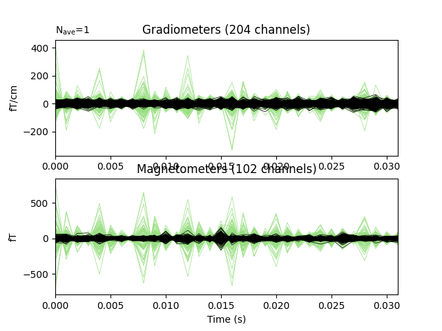
Do a quick visualization of how much variance we explained, putting the data and residuals on the same scale (here the “time points” are the 32 dipole peak values that we fit):
fig, axes = plt.subplots(2, 1)
evoked.plot(axes=axes)
for ax in axes:
    for text in list(ax.texts):
        text.remove()
    for line in ax.lines:
        line.set_color('#98df81')
residual.plot(axes=axes)
Now we can compare to the actual locations, taking the difference in mm:
actual_pos, actual_ori = mne.dipole.get_phantom_dipoles()
actual_amp = 100.  # nAm

fig, (ax1, ax2, ax3) = plt.subplots(nrows=3, ncols=1, figsize=(6, 7))

diffs = 1000 * np.sqrt(np.sum((dip.pos - actual_pos) ** 2, axis=-1))
print('mean(position error) = %0.1f mm' % (np.mean(diffs),))
ax1.bar(event_id, diffs)
ax1.set_xlabel('Dipole index')
ax1.set_ylabel('Loc. error (mm)')

angles = np.rad2deg(np.arccos(np.abs(np.sum(dip.ori * actual_ori, axis=1))))
print(u'mean(angle error) = %0.1f°' % (np.mean(angles),))
ax2.bar(event_id, angles)
ax2.set_xlabel('Dipole index')
ax2.set_ylabel(u'Angle error (°)')

amps = actual_amp - dip.amplitude / 1e-9
print('mean(abs amplitude error) = %0.1f nAm' % (np.mean(np.abs(amps)),))
ax3.bar(event_id, amps)
ax3.set_xlabel('Dipole index')
ax3.set_ylabel('Amplitude error (nAm)')

fig.tight_layout()
plt.show()
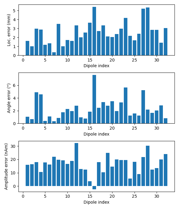
mean(position error) = 2.6 mm
mean(angle error) = 2.4°
mean(abs amplitude error) = 16.8 nAm
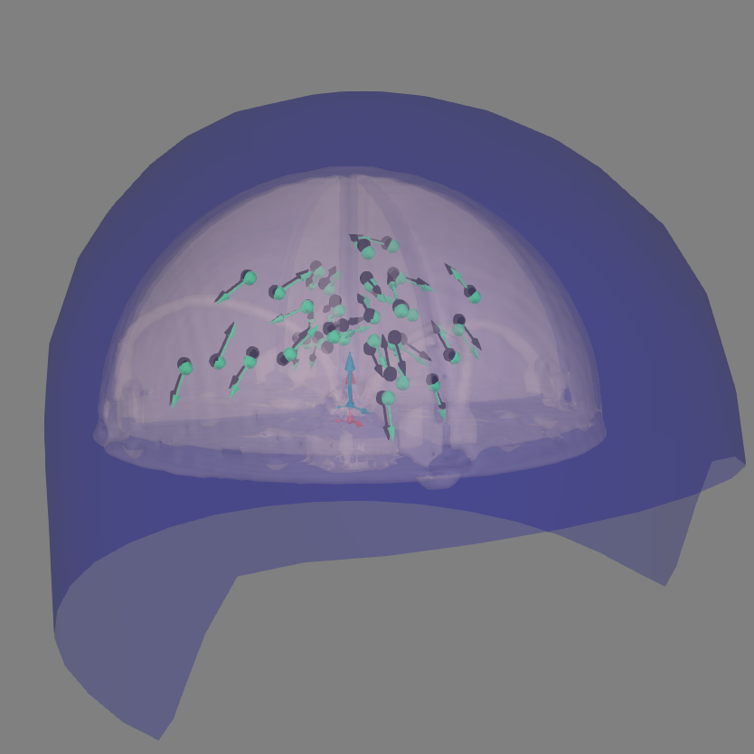
Let’s plot the positions and the orientations of the actual and the estimated dipoles
actual_amp = np.ones(len(dip))  # misc amp to create Dipole instance
actual_gof = np.ones(len(dip))  # misc GOF to create Dipole instance
dip_true = \
    mne.Dipole(dip.times, actual_pos, actual_amp, actual_ori, actual_gof)

fig = mne.viz.plot_alignment(
    evoked.info, trans, subject, bem=sphere, surfaces={'head-dense': 0.2},
    coord_frame='head', meg='helmet', show_axes=True,
    subjects_dir=subjects_dir)

# Plot the position and the orientation of the actual dipole
fig = mne.viz.plot_dipole_locations(dipoles=dip_true, mode='arrow',
                                    subject=subject, color=(0., 0., 0.),
                                    fig=fig)

# Plot the position and the orientation of the estimated dipole
fig = mne.viz.plot_dipole_locations(dipoles=dip, mode='arrow', subject=subject,
                                    color=(0.2, 1., 0.5), fig=fig)

mne.viz.set_3d_view(figure=fig, azimuth=70, elevation=80, distance=0.5)
Using lh.seghead for head surface.
Getting helmet for system 306m
References#
- 1
François Tadel, Sylvain Baillet, John C. Mosher, Dimitrios Pantazis, and Richard M. Leahy. Brainstorm: a user-friendly application for MEG/EEG analysis. Computational Intelligence and Neuroscience, 2011:1–13, 2011. doi:10.1155/2011/879716.
Total running time of the script: ( 0 minutes 45.389 seconds)
Estimated memory usage: 185 MB