mne.viz.plot_filter#
- mne.viz.plot_filter(h, sfreq, freq=None, gain=None, title=None, color='#1f77b4', flim=None, fscale='log', alim=(-80, 10), show=True, compensate=False, plot=('time', 'magnitude', 'delay'), axes=None, *, dlim=None)[source]#
Plot properties of a filter.
- Parameters:
- h
dictorndarray An IIR dict or 1D ndarray of coefficients (for FIR filter).
- sfreq
float Sample rate of the data (Hz).
- freqarray-like or
None The ideal response frequencies to plot (must be in ascending order). If None (default), do not plot the ideal response.
- gainarray-like or
None The ideal response gains to plot. If None (default), do not plot the ideal response.
- title
str|None The title to use. If None (default), determine the title based on the type of the system.
- colorcolor object
The color to use (default ‘#1f77b4’).
- flim
tupleorNone If not None, the x-axis frequency limits (Hz) to use. If None, freq will be used. If None (default) and freq is None,
(0.1, sfreq / 2.)will be used.- fscale
str Frequency scaling to use, can be “log” (default) or “linear”.
- alim
tuple The y-axis amplitude limits (dB) to use (default: (-60, 10)).
- showbool
Show figure if True (default).
- compensatebool
If True, compensate for the filter delay (phase will not be shown).
For linear-phase FIR filters, this visualizes the filter coefficients assuming that the output will be shifted by
N // 2.For IIR filters, this changes the filter coefficient display by filtering backward and forward, and the frequency response by squaring it.
New in version 0.18.
- plot
list|tuple|str A list of the requested plots from
time,magnitudeanddelay. Default is to plot all three filter properties (‘time’, ‘magnitude’, ‘delay’).New in version 0.21.0.
- axesinstance of
Axes|list|None The axes to plot to. If list, the list must be a list of Axes of the same length as the number of requested plot types. If instance of Axes, there must be only one filter property plotted. Defaults to
None.New in version 0.21.0.
- dlim
None|tuple The y-axis delay limits (sec) to use (default:
(-tmax / 2., tmax / 2.)).New in version 1.1.0.
- h
- Returns:
- fig
matplotlib.figure.Figure The figure containing the plots.
- fig
Notes
New in version 0.14.