mne.viz.plot_sparse_source_estimates#
- mne.viz.plot_sparse_source_estimates(src, stcs, colors=None, linewidth=2, fontsize=18, bgcolor=(0.05, 0, 0.1), opacity=0.2, brain_color=(0.7, 0.7, 0.7), show=True, high_resolution=False, fig_name=None, fig_number=None, labels=None, modes=('cone', 'sphere'), scale_factors=(1, 0.6), verbose=None, **kwargs)[source]#
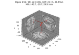
Plot source estimates obtained with sparse solver.
Active dipoles are represented in a “Glass” brain. If the same source is active in multiple source estimates it is displayed with a sphere otherwise with a cone in 3D.
- Parameters:
- src
dict The source space.
- stcsinstance of
SourceEstimateorlistof instances ofSourceEstimate The source estimates.
- colors
list List of colors.
- linewidth
int Line width in 2D plot.
- fontsize
int Font size.
- bgcolor
tupleof length 3 Background color in 3D.
- opacity
floatin [0, 1] Opacity of brain mesh.
- brain_color
tupleof length 3 Brain color.
- showbool
Show figures if True.
- high_resolutionbool
If True, plot on the original (non-downsampled) cortical mesh.
- fig_name
str PyVista figure name.
- fig_number
int Matplotlib figure number.
- labels
ndarrayorlistofndarray Labels to show sources in clusters. Sources with the same label and the waveforms within each cluster are presented in the same color. labels should be a list of ndarrays when stcs is a list ie. one label for each stc.
- modes
list Should be a list, with each entry being
'cone'or'sphere'to specify how the dipoles should be shown. The pivot for the glyphs in'cone'mode is always the tail whereas the pivot in'sphere'mode is the center.- scale_factors
list List of floating point scale factors for the markers.
- verbosebool |
str|int|None Control verbosity of the logging output. If
None, use the default verbosity level. See the logging documentation andmne.verbose()for details. Should only be passed as a keyword argument.- **kwargskwargs
Keyword arguments to pass to renderer.mesh.
- src
- Returns:
- surfaceinstance of
Figure3D The 3D figure containing the triangular mesh surface.
- surfaceinstance of
Examples using mne.viz.plot_sparse_source_estimates#
Compute a sparse inverse solution using the Gamma-MAP empirical Bayesian method
Compute sparse inverse solution with mixed norm: MxNE and irMxNE
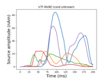
Compute iterative reweighted TF-MxNE with multiscale time-frequency dictionary