mne.time_frequency.tfr_multitaper#
- mne.time_frequency.tfr_multitaper(inst, freqs, n_cycles, time_bandwidth=4.0, use_fft=True, return_itc=True, decim=1, n_jobs=None, picks=None, average=True, *, verbose=None)[source]#
Warning
LEGACY: New code should use .compute_tfr(method=”multitaper”).
Compute Time-Frequency Representation (TFR) using DPSS tapers.
Same computation as
tfr_array_multitaper(), but operates onEpochsorEvokedobjects instead ofNumPy arrays.- Parameters:
- inst
Epochs|Evoked The epochs or evoked object.
- freqs
ndarray, shape (n_freqs,) The frequencies in Hz.
- n_cycles
int|arrayofint, shape (n_freqs,) Number of cycles in the wavelet, either a fixed number or one per frequency. The number of cycles
n_cyclesand the frequencies of interestfreqsdefine the temporal window length. See notes for additional information about the relationship between those arguments and about time and frequency smoothing.- time_bandwidth
float≥ 2.0 Product between the temporal window length (in seconds) and the full frequency bandwidth (in Hz). This product can be seen as the surface of the window on the time/frequency plane and controls the frequency bandwidth (thus the frequency resolution) and the number of good tapers. See notes for additional information.
- use_fftbool, default
True The fft based convolution or not.
- return_itcbool, default
True Return inter-trial coherence (ITC) as well as averaged (or single-trial) power.
- decim
int|slice Decimation factor, applied after time-frequency decomposition.
if
int, returnstfr[..., ::decim](keep only every Nth sample along the time axis).if
slice, returnstfr[..., decim](keep only the specified slice along the time axis).
Note
Decimation is done after convolutions and may create aliasing artifacts.
- n_jobs
int|None The number of jobs to run in parallel. If
-1, it is set to the number of CPU cores. Requires thejoblibpackage.None(default) is a marker for ‘unset’ that will be interpreted asn_jobs=1(sequential execution) unless the call is performed under ajoblib.parallel_configcontext manager that sets another value forn_jobs.- picks
str| array_like |slice|None Channels to include. Slices and lists of integers will be interpreted as channel indices. In lists, channel type strings (e.g.,
['meg',
'eeg']
) will pick channels of those types, channel name strings (e.g.,['MEG0111', 'MEG2623']will pick the given channels. Can also be the string values'all'to pick all channels, or'data'to pick data channels. None (default) will pick good data channels. Note that channels ininfo['bads']will be included if their names or indices are explicitly provided.- averagebool, default
True If
Falsereturn anEpochsTFRcontaining separate TFRs for each epoch. IfTruereturn anAverageTFRcontaining the average of all TFRs across epochs.Note
Using
average=Trueis functionally equivalent to usingaverage=Falsefollowed byEpochsTFR.average(), but is more memory efficient.New in v0.13.0.
- verbosebool |
str|int|None Control verbosity of the logging output. If
None, use the default verbosity level. See the logging documentation andmne.verbose()for details. Should only be passed as a keyword argument.
- inst
- Returns:
- power
AverageTFR|EpochsTFR The averaged or single-trial power.
- itc
AverageTFR|EpochsTFR The inter-trial coherence (ITC). Only returned if return_itc is True.
- power
See also
Notes
In spectrotemporal analysis (as with traditional fourier methods), the temporal and spectral resolution are interrelated: longer temporal windows allow more precise frequency estimates; shorter temporal windows “smear” frequency estimates while providing more precise timing information.
Time-frequency representations are computed using a sliding temporal window. Either the temporal window has a fixed length independent of frequency, or the temporal window decreases in length with increased frequency.
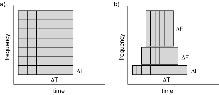
Figure: Time and frequency smoothing. (a) For a fixed length temporal window the time and frequency smoothing remains fixed. (b) For temporal windows that decrease with frequency, the temporal smoothing decreases and the frequency smoothing increases with frequency. Source: FieldTrip tutorial: Time-frequency analysis using Hanning window, multitapers and wavelets.
In MNE-Python, the multitaper temporal window length is defined by the arguments
freqsandn_cycles, respectively defining the frequencies of interest and the number of cycles: \(T = \frac{\mathtt{n\_cycles}}{\mathtt{freqs}}\)A fixed number of cycles for all frequencies will yield a temporal window which decreases with frequency. For example,
freqs=np.arange(1, 6, 2)andn_cycles=2yieldsT=array([2., 0.7, 0.4]).To use a temporal window with fixed length, the number of cycles has to be defined based on the frequency. For example,
freqs=np.arange(1, 6, 2)andn_cycles=freqs / 2yieldsT=array([0.5, 0.5, 0.5]).In MNE-Python’s multitaper functions, the frequency bandwidth is additionally affected by the parameter
time_bandwidth. Then_cyclesparameter determines the temporal window length based on the frequencies of interest: \(T = \frac{\mathtt{n\_cycles}}{\mathtt{freqs}}\). Thetime_bandwidthparameter defines the “time-bandwidth product”, which is the product of the temporal window length (in seconds) and the frequency bandwidth (in Hz). Thus oncen_cycleshas been set, frequency bandwidth is determined by \(\frac{\mathrm{time~bandwidth}}{\mathrm{time~window}}\), and thus passing a largertime_bandwidthvalue will increase the frequency bandwidth (thereby decreasing the frequency resolution).The increased frequency bandwidth is reached by averaging spectral estimates obtained from multiple tapers. Thus,
time_bandwidthalso determines the number of tapers used. MNE-Python uses only “good” tapers (tapers with minimal leakage from far-away frequencies); the number of good tapers isfloor(time_bandwidth - 1). This means there is another trade-off at play, between frequency resolution and the variance reduction that multitaper analysis provides. Striving for finer frequency resolution (by settingtime_bandwidthlow) means fewer tapers will be used, which undermines what is unique about multitaper methods — namely their ability to improve accuracy / reduce noise in the power estimates by using several (orthogonal) tapers.Warning
In
tfr_array_multitaperandtfr_multitaper,time_bandwidthdefines the product of the temporal window length with the full frequency bandwidth For example, a full bandwidth of 4 Hz at a frequency of interest of 10 Hz will “smear” the frequency estimate between 8 Hz and 12 Hz.This is not the case for
psd_array_multitaperwhere the argumentbandwidthdefines the half frequency bandwidth. In the example above, the half-frequency bandwidth is 2 Hz.New in v0.9.0.
Examples using mne.time_frequency.tfr_multitaper#
Time-frequency on simulated data (Multitaper vs. Morlet vs. Stockwell vs. Hilbert)