mne.time_frequency.tfr_morlet#
- mne.time_frequency.tfr_morlet(inst, freqs, n_cycles, use_fft=False, return_itc=True, decim=1, n_jobs=None, picks=None, zero_mean=True, average=True, output='power', verbose=None)[source]#
Warning
LEGACY: New code should use .compute_tfr(method=”morlet”).
Compute Time-Frequency Representation (TFR) using Morlet wavelets.
Same computation as
tfr_array_morlet, but operates onEpochsorEvokedobjects instead ofNumPy arrays.- Parameters:
- inst
Epochs|Evoked The epochs or evoked object.
- freqs
ndarray, shape (n_freqs,) The frequencies in Hz.
- n_cycles
int|arrayofint, shape (n_freqs,) Number of cycles in the wavelet, either a fixed number or one per frequency. The number of cycles
n_cyclesand the frequencies of interestfreqsdefine the temporal window length. See notes for additional information about the relationship between those arguments and about time and frequency smoothing.- use_fftbool, default
False The fft based convolution or not.
- return_itcbool, default
True Return inter-trial coherence (ITC) as well as averaged power. Must be
Falsefor evoked data.- decim
int|slice Decimation factor, applied after time-frequency decomposition.
if
int, returnstfr[..., ::decim](keep only every Nth sample along the time axis).if
slice, returnstfr[..., decim](keep only the specified slice along the time axis).
Note
Decimation is done after convolutions and may create aliasing artifacts.
- n_jobs
int|None The number of jobs to run in parallel. If
-1, it is set to the number of CPU cores. Requires thejoblibpackage.None(default) is a marker for ‘unset’ that will be interpreted asn_jobs=1(sequential execution) unless the call is performed under ajoblib.parallel_configcontext manager that sets another value forn_jobs.- picksarray_like of
int|None, defaultNone The indices of the channels to decompose. If None, all available good data channels are decomposed.
- zero_meanbool, default
True Make sure the wavelet has a mean of zero.
New in v0.13.0.
- averagebool, default
True If
Falsereturn anEpochsTFRcontaining separate TFRs for each epoch. IfTruereturn anAverageTFRcontaining the average of all TFRs across epochs.Note
Using
average=Trueis functionally equivalent to usingaverage=Falsefollowed byEpochsTFR.average(), but is more memory efficient.New in v0.13.0.
- output
str Can be
"power"(default) or"complex". If"complex", thenaveragemust beFalse.New in v0.15.0.
- verbosebool |
str|int|None Control verbosity of the logging output. If
None, use the default verbosity level. See the logging documentation andmne.verbose()for details. Should only be passed as a keyword argument.
- inst
- Returns:
- power
AverageTFR|EpochsTFR The averaged or single-trial power.
- itc
AverageTFR|EpochsTFR The inter-trial coherence (ITC). Only returned if return_itc is True.
- power
See also
Notes
The Morlet wavelets follow the formulation in Tallon-Baudry et al.[1].
In spectrotemporal analysis (as with traditional fourier methods), the temporal and spectral resolution are interrelated: longer temporal windows allow more precise frequency estimates; shorter temporal windows “smear” frequency estimates while providing more precise timing information.
Time-frequency representations are computed using a sliding temporal window. Either the temporal window has a fixed length independent of frequency, or the temporal window decreases in length with increased frequency.
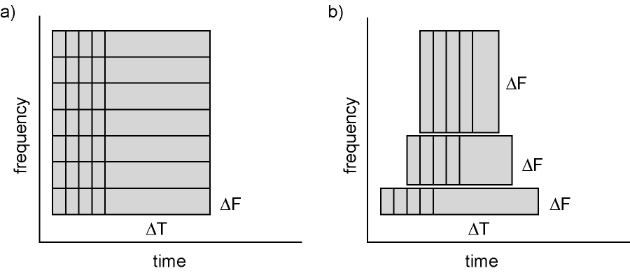
Figure: Time and frequency smoothing. (a) For a fixed length temporal window the time and frequency smoothing remains fixed. (b) For temporal windows that decrease with frequency, the temporal smoothing decreases and the frequency smoothing increases with frequency. Source: FieldTrip tutorial: Time-frequency analysis using Hanning window, multitapers and wavelets.
In MNE-Python, the length of the Morlet wavelet is affected by the arguments
freqsandn_cycles, which define the frequencies of interest and the number of cycles, respectively. For the time-frequency representation, the length of the wavelet is defined such that both tails of the wavelet extend five standard deviations from the midpoint of its Gaussian envelope and that there is a sample at time zero.The length of the wavelet is thus \(10\times\mathtt{sfreq}\cdot\sigma-1\), which is equal to \(\frac{5}{\pi} \cdot \frac{\mathtt{n\_cycles} \cdot \mathtt{sfreq}}{\mathtt{freqs}} - 1\), where \(\sigma = \frac{\mathtt{n\_cycles}}{2\pi f}\) corresponds to the standard deviation of the wavelet’s Gaussian envelope. Note that the length of the wavelet must not exceed the length of your signal.
For more information on the Morlet wavelet, see
mne.time_frequency.morlet().See
mne.time_frequency.morlet()for more information about the Morlet wavelet.References
Examples using mne.time_frequency.tfr_morlet#
Time-frequency on simulated data (Multitaper vs. Morlet vs. Stockwell vs. Hilbert)