mne.preprocessing.EOGRegression#
- class mne.preprocessing.EOGRegression(picks=None, exclude='bads', picks_artifact='eog', proj=True)[source]#
Remove EOG artifact signals from other channels by regression.
Employs linear regression to remove signals captured by some channels, typically EOG, as described in [1]. You can also choose to fit the regression coefficients on evoked blink/saccade data and then apply them to continuous data, as described in [2].
- Parameters:
- picks
str| array_like |slice|None Channels to include. Slices and lists of integers will be interpreted as channel indices. In lists, channel type strings (e.g.,
['meg',
'eeg']
) will pick channels of those types, channel name strings (e.g.,['MEG0111', 'MEG2623']will pick the given channels. Can also be the string values'all'to pick all channels, or'data'to pick data channels. None (default) will pick good data channels. Note that channels ininfo['bads']will be included if their names or indices are explicitly provided.- exclude
list| ‘bads’ List of channels to exclude from the regression, only used when picking based on types (e.g., exclude=”bads” when picks=”meg”). Specify
'bads'(the default) to exclude all channels marked as bad.- picks_artifactarray_like |
str Channel picks to use as predictor/explanatory variables capturing the artifact of interest (default is “eog”).
- projbool
Whether to automatically apply SSP projection vectors before fitting and applying the regression. Default is
True.
- picks
- Attributes:
- coef_
ndarray, shape (n, n) The regression coefficients. Only available after fitting.
- info_
Info Channel information corresponding to the regression weights. Only available after fitting.
- picksarray_like |
str Channels to perform the regression on.
- exclude
list| ‘bads’ Channels to exclude from the regression.
- picks_artifactarray_like |
str The channels designated as containing the artifacts of interest.
- projbool
Whether projections will be applied before performing the regression.
- coef_
Methods
apply(inst[, copy])Apply the regression coefficients to data.
fit(inst)Fit EOG regression coefficients.
plot([ch_type, sensors, show_names, mask, ...])Plot the regression weights of a fitted EOGRegression model.
save(fname[, overwrite])Save the regression model to an HDF5 file.
Notes
New in v1.2.
References
- apply(inst, copy=True)[source]#
Apply the regression coefficients to data.
- Parameters:
- Returns:
Notes
Only works after
.fit()has been used.References
Examples using
apply:
Preprocessing optically pumped magnetometer (OPM) MEG data
Preprocessing optically pumped magnetometer (OPM) MEG data
- fit(inst)[source]#
Fit EOG regression coefficients.
- Parameters:
- Returns:
- self
EOGRegression The fitted
EOGRegressionobject. The regression coefficients are available as the.coef_and.intercept_attributes.
- self
Notes
If your data contains EEG channels, make sure to apply the desired reference (see
mne.set_eeg_reference()) before performing EOG regression.Examples using
fit:
Preprocessing optically pumped magnetometer (OPM) MEG data
Preprocessing optically pumped magnetometer (OPM) MEG data
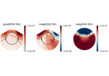
- plot(ch_type=None, sensors=True, show_names=False, mask=None, mask_params=None, mask_label_params=None, contours=6, outlines='head', sphere=None, image_interp='cubic', extrapolate='auto', border='mean', res=64, size=1, cmap=None, vlim=(None, None), cnorm=None, axes=None, colorbar=True, cbar_fmt='%1.1e', title=None, show=True)[source]#
Plot the regression weights of a fitted EOGRegression model.
- Parameters:
- ch_type‘mag’ | ‘grad’ | ‘planar1’ | ‘planar2’ | ‘eeg’ |
None The channel type to plot. For
'grad', the gradiometers are collected in pairs and the RMS for each pair is plotted. IfNonethe first available channel type from order shown above is used. Defaults toNone.- sensorsbool |
str Whether to add markers for sensor locations. If
str, should be a valid matplotlib format string (e.g.,'r+'for red plusses, see the Notes section ofplot()). IfTrue(the default), black circles will be used.- show_namesbool |
callable() If
True, show channel names next to each sensor marker. If callable, channel names will be formatted using the callable; e.g., to delete the prefix ‘MEG ‘ from all channel names, pass the functionlambda x: x.replace('MEG ', ''). Ifmaskis notNone, only non-masked sensor names will be shown.- mask
ndarrayof bool, shape (n_channels,) |None Array indicating channel(s) to highlight with a distinct plotting style. Array elements set to
Truewill be plotted with the parameters given inmask_params. Defaults toNone, equivalent to an array of allFalseelements.- mask_params
dict|None Additional plotting parameters for plotting significant sensors. Default (None) equals:
dict(marker='o', markerfacecolor='w', markeredgecolor='k',
        linewidth=0, markersize=4)
- mask_label_params
dict|None Additional plotting parameters for significant sensor labels. Default (None) equals:
dict(fontsize='medium', fontweight='bold')
New in v1.13.
- contours
int| array_like The number of contour lines to draw. If
0, no contours will be drawn. If a positive integer, that number of contour levels are chosen using the matplotlib tick locator (may sometimes be inaccurate, use array for accuracy). If array-like, the array values are used as the contour levels. The values should be in µV for EEG, fT for magnetometers and fT/m for gradiometers. Ifcolorbar=True, the colorbar will have ticks corresponding to the contour levels. Default is6.- outlines‘head’ |
dict|None The outlines to be drawn. If ‘head’, the default head scheme will be drawn. If dict, each key refers to a tuple of x and y positions, the values in ‘mask_pos’ will serve as image mask. Alternatively, a matplotlib patch object can be passed for advanced masking options, either directly or as a function that returns patches (required for multi-axis plots). If None, nothing will be drawn. Defaults to ‘head’.
- sphere
float| array_like offloat| instance ofConductorModel|str|listofstr|None The sphere parameters to use for the head outline. Can be array-like of shape (4,) to give the X/Y/Z origin and radius in meters, or a single float to give just the radius (origin assumed 0, 0, 0). Can also be an instance of a spherical
ConductorModelto use the origin and radius from that object. Can also be astr, in which case:'auto': the sphere is fit to external digitization points first, and to external + EEG digitization points if the former fails.'eeglab': the head circle is defined by EEG electrodes'Fpz','Oz','T7', and'T8'(if'Fpz'is not present, it will be approximated from the coordinates of'Oz').'extra': the sphere is fit to external digitization points.'eeg': the sphere is fit to EEG digitization points.'cardinal': the sphere is fit to cardinal digitization points.'hpi': the sphere is fit to HPI coil digitization points.
Can also be a list of
str, in which case the sphere is fit to the specified digitization points, which can be any combination of'extra','eeg','cardinal', and'hpi', as specified above.None(the default) is equivalent to'auto'when enough extra digitization points are available, and (0, 0, 0, 0.095) otherwise.New in v0.20.
Changed in version 1.1: Added
'eeglab'option.Changed in version 1.11: Added
'extra','eeg','cardinal','hpi'and list ofstroptions.- image_interp
str The image interpolation to be used. Options are
'cubic'(default) to usescipy.interpolate.CloughTocher2DInterpolator,'nearest'to usescipy.spatial.Voronoior'linear'to usescipy.interpolate.LinearNDInterpolator.- extrapolate
str Options:
'box'Extrapolate to four points placed to form a square encompassing all data points, where each side of the square is three times the range of the data in the respective dimension.
'local'(default for MEG sensors)Extrapolate only to nearby points (approximately to points closer than median inter-electrode distance). This will also set the mask to be polygonal based on the convex hull of the sensors.
'head'(default for non-MEG sensors)Extrapolate out to the edges of the clipping circle. This will be on the head circle when the sensors are contained within the head circle, but it can extend beyond the head when sensors are plotted outside the head circle.
Changed in version 0.21:
The default was changed to
'local'for MEG sensors.'local'was changed to use a convex hull mask'head'was changed to extrapolate out to the clipping circle.
- border
float| ‘mean’ Value to extrapolate to on the topomap borders. If
'mean'(default), then each extrapolated point has the average value of its neighbours.New in v0.20.
- res
int The resolution of the topomap image (number of pixels along each side).
- size
float Side length of each subplot in inches.
- cmap
str|matplotlib.colors.Colormap|tuple| ‘interactive’ |None Colormap to use. If
tuple, the first value indicates the colormap to use and the second value is a boolean defining interactivity. In interactive mode the colors are adjustable by clicking and dragging the colorbar with left and right mouse button. Left mouse button moves the scale up and down and right mouse button adjusts the range. Hitting space bar resets the range. Up and down arrows can be used to change the colormap. IfNone,'Reds'is used for data that is either all-positive or all-negative, and'RdBu_r'is used otherwise.'interactive'is equivalent to(None, True). Defaults toNone.Warning
Interactive mode works smoothly only for a small amount of topomaps. Interactive mode is disabled by default for more than 2 topomaps.
- vlim
tupleof length 2 Lower and upper bounds of the colormap, typically a numeric value in the same units as the data. If both entries are
None, the bounds are set at(min(data), max(data)). ProvidingNonefor just one entry will set the corresponding boundary at the min/max of the data. Defaults to(None, None).- cnorm
matplotlib.colors.Normalize|None How to normalize the colormap. If
None, standard linear normalization is performed. If notNone,vminandvmaxwill be ignored. See Matplotlib docs for more details on colormap normalization, and the ERDs example for an example of its use.- axesinstance of
Axes|listofAxes|None The axes to plot into. If
None, a newFigurewill be created with the correct number of axes. IfAxesare provided (either as a single instance or alistof axes), the number of axes provided must match the number oftimesprovided (unlesstimesisNone). Default isNone.- colorbarbool
Plot a colorbar in the rightmost column of the figure.
- cbar_fmt
str Formatting string for colorbar tick labels. See Format specification mini-language for details.
- title
str|None The title of the generated figure. If
None(default), no title is displayed.- showbool
Show the figure if
True. When shown, blocking followsmatplotlib.pyplot.show(): the call blocks until the window is closed unless Matplotlib’s interactive mode is on (enabled withmatplotlib.pyplot.ion()or IPython’s%%matplotlibmagic command), in which case it returns immediately. Interactive mode is off by default, so a plain script or REPL blocks. Passshow=Falseto build several figures and display them together with a singlematplotlib.pyplot.show()call.
- ch_type‘mag’ | ‘grad’ | ‘planar1’ | ‘planar2’ | ‘eeg’ |
- Returns:
- figinstance of
matplotlib.figure.Figure Figure with a topomap subplot for each channel type.
- figinstance of
Notes
New in v1.2.
Examples using
plot:
Examples using mne.preprocessing.EOGRegression#
Preprocessing optically pumped magnetometer (OPM) MEG data