mne.decoding.SpatialFilter#

class mne.decoding.SpatialFilter(info, filters, *, evals=None, patterns=None, patterns_method='pinv')[source]#

Container for spatial filter weights (evecs) and patterns.

Warning

For MNE-Python decoding classes, this container should be instantiated with mne.decoding.get_spatial_filter_from_estimator. Direct instantiation with external spatial filters is possible at your own risk.

This object is obtained either by generalized eigendecomposition (GED) algorithms such as mne.decoding.CSP, mne.decoding.SPoC, mne.decoding.SSD, mne.decoding.XdawnTransformer or by mne.decoding.LinearModel, wrapping linear models like SVM or Logit. The object stores the filters that projects sensor data to a reduced component space, and the corresponding patterns (obtained by pseudoinverse in GED case or Haufe’s trick in case of mne.decoding.LinearModel). It can also be directly initialized using filters from other transformers (e.g. PyRiemann), but make sure that the dimensions match.

Parameters:

infoinstance of Info: The measurement info containing channel topography.
filtersndarray, shape ((n_classes), n_components, n_channels): The spatial filters (transposed eigenvectors of the decomposition).
evalsndarray, shape ((n_classes), n_components) | None: The eigenvalues of the decomposition. Defaults to None.
patternsndarray, shape ((n_classes), n_components, n_channels) | None: The patterns of the decomposition. If None, they will be computed from the filters using pseudoinverse. Defaults to None.
patterns_methodstr: The method used to compute the patterns. Can be 'pinv' or 'haufe'. If patterns is None, it will be set to 'pinv'. Defaults to 'pinv'.

Attributes:

infoinstance of Info: The measurement info.
filtersndarray, shape (n_components, n_channels): The spatial filters (unmixing matrix). Applying these filters to the data gives the component time series.
patternsndarray, shape (n_components, n_channels): The spatial patterns (mixing matrix/forward model). These represent the scalp topography of each component.
evalsndarray, shape (n_components,): The eigenvalues associated with each component.
patterns_methodstr: The method used to compute the patterns from the filters.

Methods

`plot_filters`([components, tmin, ch_type, ...])	Plot topographic maps of model filters.
`plot_patterns`([components, tmin, ch_type, ...])	Plot topographic maps of model patterns.
`plot_scree`([title, add_cumul_evals, axes, show])	Plot scree for GED eigenvalues.

See also

get_spatial_filter_from_estimator, mne.decoding.LinearModel, mne.decoding.CSP
mne.decoding.SSD, mne.decoding.XdawnTransformer, mne.decoding.SPoC

Notes

The spatial filters and patterns are stored with shape (n_components, n_channels).

Filters and patterns are related by the following equation:

\[\mathbf{A} = \mathbf{W}^{-1}\]

where \(\mathbf{A}\) is the matrix of patterns (the mixing matrix) and \(\mathbf{W}\) is the matrix of filters (the unmixing matrix).

For a detailed discussion on the difference between filters and patterns for GED see [1] and for linear models in general see [2].

New in v1.11.

References

plot_filters(components=None, tmin=None, *, ch_type=None, scalings=None, sensors=True, show_names=False, mask=None, mask_params=None, contours=6, outlines='head', sphere=None, image_interp='cubic', extrapolate='auto', border='mean', res=64, size=1, cmap='RdBu_r', vlim=(None, None), cnorm=None, colorbar=True, cbar_fmt='%3.1f', units=None, axes=None, name_format='Filter%01d', nrows=1, ncols='auto', show=True)[source]#

Plot topographic maps of model filters.

Parameters:

componentsfloat | array of float | ‘auto’ | None

Indices of filters to plot. If “auto”, the number of axes determines the amount of filters. If None, all filters will be plotted. Defaults to None.

tminfloat | None

In case filters are distributed temporally, this can be used to align them with times and frequency. Use epochs.tmin, for example. Defaults to None.

The channel type to plot. For 'grad', the gradiometers are collected in pairs and the RMS for each pair is plotted. If None the first available channel type from order shown above is used. Defaults to None.

scalingsdict | float | None

The scalings of the channel types to be applied for plotting. If None, defaults to dict(eeg=1e6, grad=1e13, mag=1e15).

sensorsbool | str

Whether to add markers for sensor locations. If str, should be a valid matplotlib format string (e.g., 'r+' for red plusses, see the Notes section of plot()). If True (the default), black circles will be used.

show_namesbool | callable()

If True, show channel names next to each sensor marker. If callable, channel names will be formatted using the callable; e.g., to delete the prefix ‘MEG ‘ from all channel names, pass the function lambda x: x.replace('MEG ', ''). If mask is not None, only non-masked sensor names will be shown.

maskndarray of bool, shape (n_channels, n_times) | None

Array indicating channel-time combinations to highlight with a distinct plotting style (useful for, e.g. marking which channels at which times a statistical test of the data reaches significance). Array elements set to True will be plotted with the parameters given in mask_params. Defaults to None, equivalent to an array of all False elements.

mask_paramsdict | None

Additional plotting parameters for plotting significant sensors. Default (None) equals:

dict(marker='o', markerfacecolor='w', markeredgecolor='k',
        linewidth=0, markersize=4)

contoursint | array_like

The number of contour lines to draw. If 0, no contours will be drawn. If a positive integer, that number of contour levels are chosen using the matplotlib tick locator (may sometimes be inaccurate, use array for accuracy). If array-like, the array values are used as the contour levels. The values should be in µV for EEG, fT for magnetometers and fT/m for gradiometers. If colorbar=True, the colorbar will have ticks corresponding to the contour levels. Default is 6.

outlines‘head’ | dict | None

The outlines to be drawn. If ‘head’, the default head scheme will be drawn. If dict, each key refers to a tuple of x and y positions, the values in ‘mask_pos’ will serve as image mask. Alternatively, a matplotlib patch object can be passed for advanced masking options, either directly or as a function that returns patches (required for multi-axis plots). If None, nothing will be drawn. Defaults to ‘head’.

The sphere parameters to use for the head outline. Can be array-like of shape (4,) to give the X/Y/Z origin and radius in meters, or a single float to give just the radius (origin assumed 0, 0, 0). Can also be an instance of a spherical ConductorModel to use the origin and radius from that object. If 'auto' the sphere is fit to digitization points. If 'eeglab' the head circle is defined by EEG electrodes 'Fpz', 'Oz', 'T7', and 'T8' (if 'Fpz' is not present, it will be approximated from the coordinates of 'Oz'). None (the default) is equivalent to 'auto' when enough extra digitization points are available, and (0, 0, 0, 0.095) otherwise.

New in v0.20.

Changed in version 1.1: Added 'eeglab' option.

image_interpstr

The image interpolation to be used. Options are 'cubic' (default) to use scipy.interpolate.CloughTocher2DInterpolator, 'nearest' to use scipy.spatial.Voronoi or 'linear' to use scipy.interpolate.LinearNDInterpolator.

extrapolatestr

Options:

'box'
Extrapolate to four points placed to form a square encompassing all data points, where each side of the square is three times the range of the data in the respective dimension.
'local' (default for MEG sensors)
Extrapolate only to nearby points (approximately to points closer than median inter-electrode distance). This will also set the mask to be polygonal based on the convex hull of the sensors.
'head' (default for non-MEG sensors)
Extrapolate out to the edges of the clipping circle. This will be on the head circle when the sensors are contained within the head circle, but it can extend beyond the head when sensors are plotted outside the head circle.

borderfloat | ‘mean’

Value to extrapolate to on the topomap borders. If 'mean' (default), then each extrapolated point has the average value of its neighbours.

resint

The resolution of the topomap image (number of pixels along each side).

sizefloat

Side length of each subplot in inches.

cmapmatplotlib colormap | (colormap, bool) | ‘interactive’ | None

Colormap to use. If tuple, the first value indicates the colormap to use and the second value is a boolean defining interactivity. In interactive mode the colors are adjustable by clicking and dragging the colorbar with left and right mouse button. Left mouse button moves the scale up and down and right mouse button adjusts the range. Hitting space bar resets the range. Up and down arrows can be used to change the colormap. If None, 'Reds' is used for data that is either all-positive or all-negative, and 'RdBu_r' is used otherwise. 'interactive' is equivalent to (None, True). Defaults to None.

Warning

Interactive mode works smoothly only for a small amount of topomaps. Interactive mode is disabled by default for more than 2 topomaps.

vlimtuple of length 2 | “joint”

Lower and upper bounds of the colormap, typically a numeric value in the same units as the data. Elements of the tuple may also be callable functions which take in a NumPy array and return a scalar.

If both entries are None, the bounds are set at ± the maximum absolute value of the data (yielding a colormap with midpoint at 0), or (0, max(abs(data))) if the (possibly baselined) data are all-positive. Providing None for just one entry will set the corresponding boundary at the min/max of the data. If vlim="joint", will compute the colormap limits jointly across all topomaps of the same channel type (instead of separately for each topomap), using the min/max of the data for that channel type. Defaults to (None, None).

cnormmatplotlib.colors.Normalize | None

How to normalize the colormap. If None, standard linear normalization is performed. If not None, vmin and vmax will be ignored. See Matplotlib docs for more details on colormap normalization, and the ERDs example for an example of its use.

colorbarbool

Plot a colorbar in the rightmost column of the figure.

cbar_fmtstr

Formatting string for colorbar tick labels. See Format Specification Mini-Language for details.

unitsdict | str | None

The units to use for the colorbar label. Ignored if colorbar=False. If None and scalings=None the unit is automatically determined, otherwise the label will be “AU” indicating arbitrary units. Default is None.

axesinstance of Axes | list of Axes | None

The axes to plot into. If None, a new Figure will be created with the correct number of axes. If Axes are provided (either as a single instance or a list of axes), the number of axes provided must match the number of times provided (unless times is None). Default is None.

name_formatstr

String format for topomap values. Defaults to 'Filter%01d'.

nrows, ncolsint | ‘auto’

The number of rows and columns of topographies to plot. If either nrows or ncols is 'auto', the necessary number will be inferred. Defaults to nrows=1, ncols='auto'.

showbool

Show the figure if True.

Returns:

figinstance of matplotlib.figure.Figure: The figure.

Examples using plot_filters: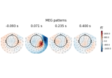

Linear classifier on sensor data with plot patterns and filters

Decoding (MVPA)

plot_patterns(components=None, tmin=None, *, ch_type=None, scalings=None, sensors=True, show_names=False, mask=None, mask_params=None, contours=6, outlines='head', sphere=None, image_interp='cubic', extrapolate='auto', border='mean', res=64, size=1, cmap='RdBu_r', vlim=(None, None), cnorm=None, colorbar=True, cbar_fmt='%3.1f', units=None, axes=None, name_format='Pattern%01d', nrows=1, ncols='auto', show=True)[source]#

Plot topographic maps of model patterns.

Parameters:

componentsfloat | array of float | ‘auto’ | None

Indices of patterns to plot. If “auto”, the number of axes determines the amount of patterns. If None, all patterns will be plotted. Defaults to None.

tminfloat | None

In case patterns are distributed temporally, this can be used to align them with times and frequency. Use epochs.tmin, for example. Defaults to None.

The channel type to plot. For 'grad', the gradiometers are collected in pairs and the RMS for each pair is plotted. If None the first available channel type from order shown above is used. Defaults to None.

scalingsdict | float | None

The scalings of the channel types to be applied for plotting. If None, defaults to dict(eeg=1e6, grad=1e13, mag=1e15).

sensorsbool | str

Whether to add markers for sensor locations. If str, should be a valid matplotlib format string (e.g., 'r+' for red plusses, see the Notes section of plot()). If True (the default), black circles will be used.

show_namesbool | callable()

If True, show channel names next to each sensor marker. If callable, channel names will be formatted using the callable; e.g., to delete the prefix ‘MEG ‘ from all channel names, pass the function lambda x: x.replace('MEG ', ''). If mask is not None, only non-masked sensor names will be shown.

maskndarray of bool, shape (n_channels, n_times) | None

Array indicating channel-time combinations to highlight with a distinct plotting style (useful for, e.g. marking which channels at which times a statistical test of the data reaches significance). Array elements set to True will be plotted with the parameters given in mask_params. Defaults to None, equivalent to an array of all False elements.

mask_paramsdict | None

Additional plotting parameters for plotting significant sensors. Default (None) equals:

dict(marker='o', markerfacecolor='w', markeredgecolor='k',
        linewidth=0, markersize=4)

contoursint | array_like

The number of contour lines to draw. If 0, no contours will be drawn. If a positive integer, that number of contour levels are chosen using the matplotlib tick locator (may sometimes be inaccurate, use array for accuracy). If array-like, the array values are used as the contour levels. The values should be in µV for EEG, fT for magnetometers and fT/m for gradiometers. If colorbar=True, the colorbar will have ticks corresponding to the contour levels. Default is 6.

outlines‘head’ | dict | None

The outlines to be drawn. If ‘head’, the default head scheme will be drawn. If dict, each key refers to a tuple of x and y positions, the values in ‘mask_pos’ will serve as image mask. Alternatively, a matplotlib patch object can be passed for advanced masking options, either directly or as a function that returns patches (required for multi-axis plots). If None, nothing will be drawn. Defaults to ‘head’.

The sphere parameters to use for the head outline. Can be array-like of shape (4,) to give the X/Y/Z origin and radius in meters, or a single float to give just the radius (origin assumed 0, 0, 0). Can also be an instance of a spherical ConductorModel to use the origin and radius from that object. If 'auto' the sphere is fit to digitization points. If 'eeglab' the head circle is defined by EEG electrodes 'Fpz', 'Oz', 'T7', and 'T8' (if 'Fpz' is not present, it will be approximated from the coordinates of 'Oz'). None (the default) is equivalent to 'auto' when enough extra digitization points are available, and (0, 0, 0, 0.095) otherwise.

New in v0.20.

Changed in version 1.1: Added 'eeglab' option.

image_interpstr

The image interpolation to be used. Options are 'cubic' (default) to use scipy.interpolate.CloughTocher2DInterpolator, 'nearest' to use scipy.spatial.Voronoi or 'linear' to use scipy.interpolate.LinearNDInterpolator.

extrapolatestr

Options:

'box'
Extrapolate to four points placed to form a square encompassing all data points, where each side of the square is three times the range of the data in the respective dimension.
'local' (default for MEG sensors)
Extrapolate only to nearby points (approximately to points closer than median inter-electrode distance). This will also set the mask to be polygonal based on the convex hull of the sensors.
'head' (default for non-MEG sensors)
Extrapolate out to the edges of the clipping circle. This will be on the head circle when the sensors are contained within the head circle, but it can extend beyond the head when sensors are plotted outside the head circle.

borderfloat | ‘mean’

Value to extrapolate to on the topomap borders. If 'mean' (default), then each extrapolated point has the average value of its neighbours.

resint

The resolution of the topomap image (number of pixels along each side).

sizefloat

Side length of each subplot in inches.

cmapmatplotlib colormap | (colormap, bool) | ‘interactive’ | None

Colormap to use. If tuple, the first value indicates the colormap to use and the second value is a boolean defining interactivity. In interactive mode the colors are adjustable by clicking and dragging the colorbar with left and right mouse button. Left mouse button moves the scale up and down and right mouse button adjusts the range. Hitting space bar resets the range. Up and down arrows can be used to change the colormap. If None, 'Reds' is used for data that is either all-positive or all-negative, and 'RdBu_r' is used otherwise. 'interactive' is equivalent to (None, True). Defaults to None.

Warning

Interactive mode works smoothly only for a small amount of topomaps. Interactive mode is disabled by default for more than 2 topomaps.

vlimtuple of length 2 | “joint”

Lower and upper bounds of the colormap, typically a numeric value in the same units as the data. Elements of the tuple may also be callable functions which take in a NumPy array and return a scalar.

If both entries are None, the bounds are set at ± the maximum absolute value of the data (yielding a colormap with midpoint at 0), or (0, max(abs(data))) if the (possibly baselined) data are all-positive. Providing None for just one entry will set the corresponding boundary at the min/max of the data. If vlim="joint", will compute the colormap limits jointly across all topomaps of the same channel type (instead of separately for each topomap), using the min/max of the data for that channel type. Defaults to (None, None).

cnormmatplotlib.colors.Normalize | None

How to normalize the colormap. If None, standard linear normalization is performed. If not None, vmin and vmax will be ignored. See Matplotlib docs for more details on colormap normalization, and the ERDs example for an example of its use.

colorbarbool

Plot a colorbar in the rightmost column of the figure.

cbar_fmtstr

Formatting string for colorbar tick labels. See Format Specification Mini-Language for details.

unitsdict | str | None

The units to use for the colorbar label. Ignored if colorbar=False. If None and scalings=None the unit is automatically determined, otherwise the label will be “AU” indicating arbitrary units. Default is None.

axesinstance of Axes | list of Axes | None

The axes to plot into. If None, a new Figure will be created with the correct number of axes. If Axes are provided (either as a single instance or a list of axes), the number of axes provided must match the number of times provided (unless times is None). Default is None.

name_formatstr

String format for topomap values. Defaults to 'Pattern%01d'.

nrows, ncolsint | ‘auto’

The number of rows and columns of topographies to plot. If either nrows or ncols is 'auto', the necessary number will be inferred. Defaults to nrows=1, ncols='auto'.

showbool

Show the figure if True.

Returns:

figinstance of matplotlib.figure.Figure: The figure.

Examples using plot_patterns: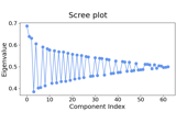

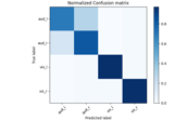
Motor imagery decoding from EEG data using the Common Spatial Pattern (CSP)

Continuous Target Decoding with SPoC

XDAWN Decoding From EEG data

Linear classifier on sensor data with plot patterns and filters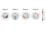

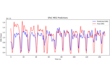
Compute spatial filters with Spatio-Spectral Decomposition (SSD)

Decoding (MVPA)

plot_scree(title='Scree plot', add_cumul_evals=False, axes=None, show=True)[source]#

Plot scree for GED eigenvalues.

Parameters:

titlestr: Title for the plot. Defaults to 'Scree plot'.
add_cumul_evalsbool: Whether to add second line and y-axis for cumulative eigenvalues. Defaults to True.
axesinstance of Axes | None: The matplotlib axes to plot to. Defaults to None.
showbool: Show the figure if True.

Returns:

figinstance of matplotlib.figure.Figure: The figure.

Examples using plot_scree:

Motor imagery decoding from EEG data using the Common Spatial Pattern (CSP)

Continuous Target Decoding with SPoC

XDAWN Decoding From EEG data

Decoding (MVPA)

Examples using `mne.decoding.SpatialFilter`#

Motor imagery decoding from EEG data using the Common Spatial Pattern (CSP)

Continuous Target Decoding with SPoC

XDAWN Decoding From EEG data

Linear classifier on sensor data with plot patterns and filters

Compute spatial filters with Spatio-Spectral Decomposition (SSD)

Decoding (MVPA)

mne.decoding.SpatialFilter#

Examples using mne.decoding.SpatialFilter#

Examples using `mne.decoding.SpatialFilter`#