Decoding (MVPA)

Design philosophy

Decoding (a.k.a. MVPA) in MNE largely follows the machine learning API of the scikit-learn package. Each estimator implements fit, transform, fit_transform, and (optionally) inverse_transform methods. For more details on this design, visit scikit-learn. For additional theoretical insights into the decoding framework in MNE [1].

For ease of comprehension, we will denote instantiations of the class using the same name as the class but in small caps instead of camel cases.

Let’s start by loading data for a simple two-class problem:

import matplotlib.pyplot as plt
import numpy as np
from sklearn.linear_model import LogisticRegression
from sklearn.pipeline import make_pipeline
from sklearn.preprocessing import StandardScaler

import mne
from mne.datasets import sample
from mne.decoding import (
    CSP,
    GeneralizingEstimator,
    LinearModel,
    Scaler,
    SlidingEstimator,
    Vectorizer,
    cross_val_multiscore,
    get_coef,
)

data_path = sample.data_path()

subjects_dir = data_path / "subjects"
meg_path = data_path / "MEG" / "sample"
raw_fname = meg_path / "sample_audvis_filt-0-40_raw.fif"
tmin, tmax = -0.200, 0.500
event_id = {"Auditory/Left": 1, "Visual/Left": 3}  # just use two
raw = mne.io.read_raw_fif(raw_fname)
raw.pick(picks=["grad", "stim", "eog"])

# The subsequent decoding analyses only capture evoked responses, so we can
# low-pass the MEG data. Usually a value more like 40 Hz would be used,
# but here low-pass at 20 so we can more heavily decimate, and allow
# the example to run faster. The 2 Hz high-pass helps improve CSP.
raw.load_data().filter(2, 20)
events = mne.find_events(raw, "STI 014")

# Set up bad channels (modify to your needs)
raw.info["bads"] += ["MEG 2443"]  # bads + 2 more

# Read epochs
epochs = mne.Epochs(
    raw,
    events,
    event_id,
    tmin,
    tmax,
    proj=True,
    picks=("grad", "eog"),
    baseline=(None, 0.0),
    preload=True,
    reject=dict(grad=4000e-13, eog=150e-6),
    decim=3,
    verbose="error",
)
epochs.pick(picks="meg", exclude="bads")  # remove stim and EOG
del raw

X = epochs.get_data(copy=False)  # MEG signals: n_epochs, n_meg_channels, n_times
y = epochs.events[:, 2]  # target: auditory left vs visual left

Opening raw data file /home/circleci/mne_data/MNE-sample-data/MEG/sample/sample_audvis_filt-0-40_raw.fif...
    Read a total of 4 projection items:
        PCA-v1 (1 x 102)  idle
        PCA-v2 (1 x 102)  idle
        PCA-v3 (1 x 102)  idle
        Average EEG reference (1 x 60)  idle
    Range : 6450 ... 48149 =     42.956 ...   320.665 secs
Ready.
Reading 0 ... 41699  =      0.000 ...   277.709 secs...
Filtering raw data in 1 contiguous segment
Setting up band-pass filter from 2 - 20 Hz

FIR filter parameters
---------------------
Designing a one-pass, zero-phase, non-causal bandpass filter:
- Windowed time-domain design (firwin) method
- Hamming window with 0.0194 passband ripple and 53 dB stopband attenuation
- Lower passband edge: 2.00
- Lower transition bandwidth: 2.00 Hz (-6 dB cutoff frequency: 1.00 Hz)
- Upper passband edge: 20.00 Hz
- Upper transition bandwidth: 5.00 Hz (-6 dB cutoff frequency: 22.50 Hz)
- Filter length: 249 samples (1.658 s)

[Parallel(n_jobs=1)]: Done  17 tasks      | elapsed:    0.0s
[Parallel(n_jobs=1)]: Done  71 tasks      | elapsed:    0.1s
[Parallel(n_jobs=1)]: Done 161 tasks      | elapsed:    0.2s
319 events found on stim channel STI 014
Event IDs: [ 1  2  3  4  5 32]

Transformation classes

Scaler

The mne.decoding.Scaler will standardize the data based on channel scales. In the simplest modes scalings=None or scalings=dict(...), each data channel type (e.g., mag, grad, eeg) is treated separately and scaled by a constant. This is the approach used by e.g., mne.compute_covariance() to standardize channel scales.

If scalings='mean' or scalings='median', each channel is scaled using empirical measures. Each channel is scaled independently by the mean and standand deviation, or median and interquartile range, respectively, across all epochs and time points during fit (during training). The transform() method is called to transform data (training or test set) by scaling all time points and epochs on a channel-by-channel basis. To perform both the fit and transform operations in a single call, the fit_transform() method may be used. To invert the transform, inverse_transform() can be used. For scalings='median', scikit-learn version 0.17+ is required.

Note

Using this class is different from directly applying sklearn.preprocessing.StandardScaler or sklearn.preprocessing.RobustScaler offered by scikit-learn. These scale each classification feature, e.g. each time point for each channel, with mean and standard deviation computed across epochs, whereas mne.decoding.Scaler scales each channel using mean and standard deviation computed across all of its time points and epochs.

Vectorizer

Scikit-learn API provides functionality to chain transformers and estimators by using sklearn.pipeline.Pipeline. We can construct decoding pipelines and perform cross-validation and grid-search. However scikit-learn transformers and estimators generally expect 2D data (n_samples * n_features), whereas MNE transformers typically output data with a higher dimensionality (e.g. n_samples * n_channels * n_frequencies * n_times). A Vectorizer therefore needs to be applied between the MNE and the scikit-learn steps like:

# Uses all MEG sensors and time points as separate classification
# features, so the resulting filters used are spatio-temporal
clf = make_pipeline(
    Scaler(epochs.info),
    Vectorizer(),
    LogisticRegression(solver="liblinear"),  # liblinear is faster than lbfgs
)

scores = cross_val_multiscore(clf, X, y, cv=5, n_jobs=None)

# Mean scores across cross-validation splits
score = np.mean(scores, axis=0)
print(f"Spatio-temporal: {100 * score:0.1f}%")

Spatio-temporal: 99.2%

PSDEstimator

The mne.decoding.PSDEstimator computes the power spectral density (PSD) using the multitaper method. It takes a 3D array as input, converts it into 2D and computes the PSD.

FilterEstimator

The mne.decoding.FilterEstimator filters the 3D epochs data.

Spatial filters

Just like temporal filters, spatial filters provide weights to modify the data along the sensor dimension. They are popular in the BCI community because of their simplicity and ability to distinguish spatially-separated neural activity.

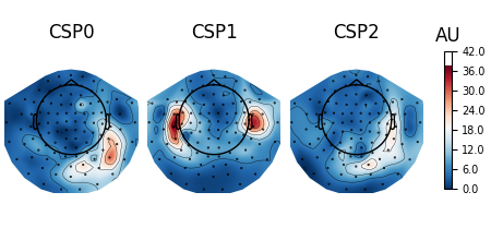
Common spatial pattern

mne.decoding.CSP is a technique to analyze multichannel data based on recordings from two classes [2] (see also https://en.wikipedia.org/wiki/Common_spatial_pattern).

Let \(X \in R^{C\times T}\) be a segment of data with \(C\) channels and \(T\) time points. The data at a single time point is denoted by \(x(t)\) such that \(X=[x(t), x(t+1), ..., x(t+T-1)]\). Common spatial pattern (CSP) finds a decomposition that projects the signal in the original sensor space to CSP space using the following transformation:

(1)\[x_{CSP}(t) = W^{T}x(t)\]

where each column of \(W \in R^{C\times C}\) is a spatial filter and each row of \(x_{CSP}\) is a CSP component. The matrix \(W\) is also called the de-mixing matrix in other contexts. Let \(\Sigma^{+} \in R^{C\times C}\) and \(\Sigma^{-} \in R^{C\times C}\) be the estimates of the covariance matrices of the two conditions. CSP analysis is given by the simultaneous diagonalization of the two covariance matrices

(2)\[W^{T}\Sigma^{+}W = \lambda^{+}\]

(3)\[W^{T}\Sigma^{-}W = \lambda^{-}\]

where \(\lambda^{C}\) is a diagonal matrix whose entries are the eigenvalues of the following generalized eigenvalue problem

(4)\[\Sigma^{+}w = \lambda \Sigma^{-}w\]

Large entries in the diagonal matrix corresponds to a spatial filter which gives high variance in one class but low variance in the other. Thus, the filter facilitates discrimination between the two classes.

Examples

• Motor imagery decoding from EEG data using the Common Spatial Pattern (CSP)

• Decoding in time-frequency space using Common Spatial Patterns (CSP)

Note

The winning entry of the Grasp-and-lift EEG competition in Kaggle used the CSP implementation in MNE and was featured as a script of the week.

We can use CSP with these data with:

csp = CSP(n_components=3, norm_trace=False)
clf_csp = make_pipeline(csp, LinearModel(LogisticRegression(solver="liblinear")))
scores = cross_val_multiscore(clf_csp, X, y, cv=5, n_jobs=None)
print(f"CSP: {100 * scores.mean():0.1f}%")

Computing rank from data with rank=None
    Using tolerance 6e-11 (2.2e-16 eps * 203 dim * 1.3e+03  max singular value)
    Estimated rank (data): 203
    data: rank 203 computed from 203 data channels with 0 projectors
Reducing data rank from 203 -> 203
Estimating class=1 covariance using EMPIRICAL
Done.
Estimating class=3 covariance using EMPIRICAL
Done.
Computing rank from data with rank=None
    Using tolerance 6e-11 (2.2e-16 eps * 203 dim * 1.3e+03  max singular value)
    Estimated rank (data): 203
    data: rank 203 computed from 203 data channels with 0 projectors
Reducing data rank from 203 -> 203
Estimating class=1 covariance using EMPIRICAL
Done.
Estimating class=3 covariance using EMPIRICAL
Done.
Computing rank from data with rank=None
    Using tolerance 6e-11 (2.2e-16 eps * 203 dim * 1.3e+03  max singular value)
    Estimated rank (data): 203
    data: rank 203 computed from 203 data channels with 0 projectors
Reducing data rank from 203 -> 203
Estimating class=1 covariance using EMPIRICAL
Done.
Estimating class=3 covariance using EMPIRICAL
Done.
Computing rank from data with rank=None
    Using tolerance 5.8e-11 (2.2e-16 eps * 203 dim * 1.3e+03  max singular value)
    Estimated rank (data): 203
    data: rank 203 computed from 203 data channels with 0 projectors
Reducing data rank from 203 -> 203
Estimating class=1 covariance using EMPIRICAL
Done.
Estimating class=3 covariance using EMPIRICAL
Done.
Computing rank from data with rank=None
    Using tolerance 5.9e-11 (2.2e-16 eps * 203 dim * 1.3e+03  max singular value)
    Estimated rank (data): 203
    data: rank 203 computed from 203 data channels with 0 projectors
Reducing data rank from 203 -> 203
Estimating class=1 covariance using EMPIRICAL
Done.
Estimating class=3 covariance using EMPIRICAL
Done.
CSP: 89.4%

Source power comodulation (SPoC)

Source Power Comodulation (mne.decoding.SPoC) [3] identifies the composition of orthogonal spatial filters that maximally correlate with a continuous target.

SPoC can be seen as an extension of the CSP where the target is driven by a continuous variable rather than a discrete variable. Typical applications include extraction of motor patterns using EMG power or audio patterns using sound envelope.

Examples

• Continuous Target Decoding with SPoC

xDAWN

mne.preprocessing.Xdawn is a spatial filtering method designed to improve the signal to signal + noise ratio (SSNR) of the ERP responses [4]. Xdawn was originally designed for P300 evoked potential by enhancing the target response with respect to the non-target response. The implementation in MNE-Python is a generalization to any type of ERP.

Examples

• XDAWN Denoising

• XDAWN Decoding From EEG data

Effect-matched spatial filtering

The result of mne.decoding.EMS is a spatial filter at each time point and a corresponding time course [5]. Intuitively, the result gives the similarity between the filter at each time point and the data vector (sensors) at that time point.

Examples

• Compute effect-matched-spatial filtering (EMS)

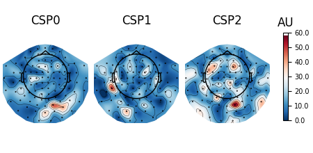
Patterns vs. filters

When interpreting the components of the CSP (or spatial filters in general), it is often more intuitive to think about how \(x(t)\) is composed of the different CSP components \(x_{CSP}(t)\). In other words, we can rewrite Equation (1) as follows:

(5)\[x(t) = (W^{-1})^{T}x_{CSP}(t)\]

The columns of the matrix \((W^{-1})^T\) are called spatial patterns. This is also called the mixing matrix. The example Linear classifier on sensor data with plot patterns and filters discusses the difference between patterns and filters.

These can be plotted with:

# Fit CSP on full data and plot
csp.fit(X, y)
csp.plot_patterns(epochs.info)
csp.plot_filters(epochs.info, scalings=1e-9)

• 
• 

Computing rank from data with rank=None
    Using tolerance 6.6e-11 (2.2e-16 eps * 203 dim * 1.5e+03  max singular value)
    Estimated rank (data): 203
    data: rank 203 computed from 203 data channels with 0 projectors
Reducing data rank from 203 -> 203
Estimating class=1 covariance using EMPIRICAL
Done.
Estimating class=3 covariance using EMPIRICAL
Done.

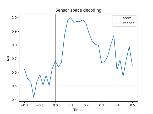
Decoding over time

This strategy consists in fitting a multivariate predictive model on each time instant and evaluating its performance at the same instant on new epochs. The mne.decoding.SlidingEstimator will take as input a pair of features \(X\) and targets \(y\), where \(X\) has more than 2 dimensions. For decoding over time the data \(X\) is the epochs data of shape n_epochs × n_channels × n_times. As the last dimension of \(X\) is the time, an estimator will be fit on every time instant.

This approach is analogous to SlidingEstimator-based approaches in fMRI, where here we are interested in when one can discriminate experimental conditions and therefore figure out when the effect of interest happens.

When working with linear models as estimators, this approach boils down to estimating a discriminative spatial filter for each time instant.

Temporal decoding

We’ll use a Logistic Regression for a binary classification as machine learning model.

# We will train the classifier on all left visual vs auditory trials on MEG

clf = make_pipeline(StandardScaler(), LogisticRegression(solver="liblinear"))

time_decod = SlidingEstimator(clf, n_jobs=None, scoring="roc_auc", verbose=True)
# here we use cv=3 just for speed
scores = cross_val_multiscore(time_decod, X, y, cv=3, n_jobs=None)

# Mean scores across cross-validation splits
scores = np.mean(scores, axis=0)

# Plot
fig, ax = plt.subplots()
ax.plot(epochs.times, scores, label="score")
ax.axhline(0.5, color="k", linestyle="--", label="chance")
ax.set_xlabel("Times")
ax.set_ylabel("AUC")  # Area Under the Curve
ax.legend()
ax.axvline(0.0, color="k", linestyle="-")
ax.set_title("Sensor space decoding")

  0%|          | Fitting SlidingEstimator : 0/36 [00:00<?,       ?it/s]
 22%|██▏       | Fitting SlidingEstimator : 8/36 [00:00<00:00,  237.10it/s]
 50%|█████     | Fitting SlidingEstimator : 18/36 [00:00<00:00,  267.56it/s]
 75%|███████▌  | Fitting SlidingEstimator : 27/36 [00:00<00:00,  267.68it/s]
100%|██████████| Fitting SlidingEstimator : 36/36 [00:00<00:00,  272.76it/s]
100%|██████████| Fitting SlidingEstimator : 36/36 [00:00<00:00,  271.61it/s]

  0%|          | Fitting SlidingEstimator : 0/36 [00:00<?,       ?it/s]
 22%|██▏       | Fitting SlidingEstimator : 8/36 [00:00<00:00,  237.07it/s]
 50%|█████     | Fitting SlidingEstimator : 18/36 [00:00<00:00,  267.53it/s]
 78%|███████▊  | Fitting SlidingEstimator : 28/36 [00:00<00:00,  276.70it/s]
100%|██████████| Fitting SlidingEstimator : 36/36 [00:00<00:00,  274.33it/s]
100%|██████████| Fitting SlidingEstimator : 36/36 [00:00<00:00,  273.38it/s]

  0%|          | Fitting SlidingEstimator : 0/36 [00:00<?,       ?it/s]
 22%|██▏       | Fitting SlidingEstimator : 8/36 [00:00<00:00,  237.07it/s]
 50%|█████     | Fitting SlidingEstimator : 18/36 [00:00<00:00,  267.82it/s]
 78%|███████▊  | Fitting SlidingEstimator : 28/36 [00:00<00:00,  278.12it/s]
100%|██████████| Fitting SlidingEstimator : 36/36 [00:00<00:00,  279.85it/s]
100%|██████████| Fitting SlidingEstimator : 36/36 [00:00<00:00,  278.49it/s]

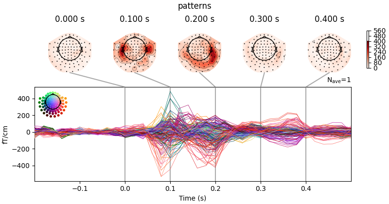
You can retrieve the spatial filters and spatial patterns if you explicitly use a LinearModel

clf = make_pipeline(
    StandardScaler(), LinearModel(LogisticRegression(solver="liblinear"))
)
time_decod = SlidingEstimator(clf, n_jobs=None, scoring="roc_auc", verbose=True)
time_decod.fit(X, y)

coef = get_coef(time_decod, "patterns_", inverse_transform=True)
evoked_time_gen = mne.EvokedArray(coef, epochs.info, tmin=epochs.times[0])
joint_kwargs = dict(ts_args=dict(time_unit="s"), topomap_args=dict(time_unit="s"))
evoked_time_gen.plot_joint(
    times=np.arange(0.0, 0.500, 0.100), title="patterns", **joint_kwargs
)

  0%|          | Fitting SlidingEstimator : 0/36 [00:00<?,       ?it/s]
 11%|█         | Fitting SlidingEstimator : 4/36 [00:00<00:00,  118.56it/s]
 25%|██▌       | Fitting SlidingEstimator : 9/36 [00:00<00:00,  133.74it/s]
 42%|████▏     | Fitting SlidingEstimator : 15/36 [00:00<00:00,  149.41it/s]
 61%|██████    | Fitting SlidingEstimator : 22/36 [00:00<00:00,  165.15it/s]
 75%|███████▌  | Fitting SlidingEstimator : 27/36 [00:00<00:00,  161.49it/s]
 92%|█████████▏| Fitting SlidingEstimator : 33/36 [00:00<00:00,  164.57it/s]
100%|██████████| Fitting SlidingEstimator : 36/36 [00:00<00:00,  165.29it/s]
100%|██████████| Fitting SlidingEstimator : 36/36 [00:00<00:00,  163.80it/s]
No projector specified for this dataset. Please consider the method self.add_proj.

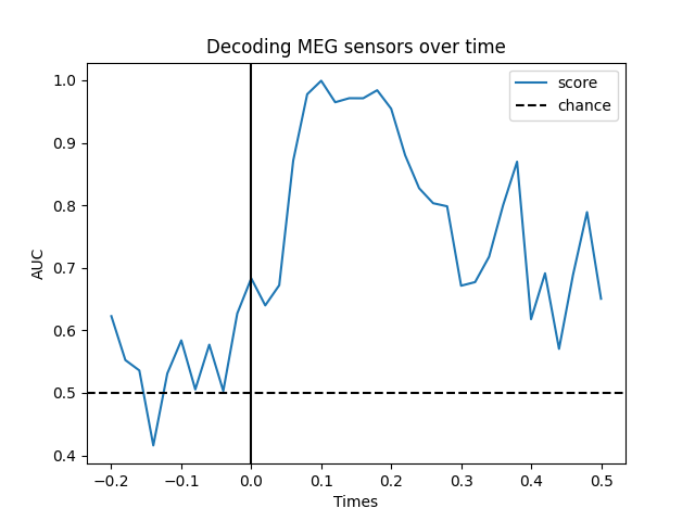
Temporal generalization

Temporal generalization is an extension of the decoding over time approach. It consists in evaluating whether the model estimated at a particular time instant accurately predicts any other time instant. It is analogous to transferring a trained model to a distinct learning problem, where the problems correspond to decoding the patterns of brain activity recorded at distinct time instants.

The object to for Temporal generalization is mne.decoding.GeneralizingEstimator. It expects as input \(X\) and \(y\) (similarly to SlidingEstimator) but generates predictions from each model for all time instants. The class GeneralizingEstimator is generic and will treat the last dimension as the one to be used for generalization testing. For convenience, here, we refer to it as different tasks. If \(X\) corresponds to epochs data then the last dimension is time.

This runs the analysis used in [6] and further detailed in [7]:

# define the Temporal generalization object
time_gen = GeneralizingEstimator(clf, n_jobs=None, scoring="roc_auc", verbose=True)

# again, cv=3 just for speed
scores = cross_val_multiscore(time_gen, X, y, cv=3, n_jobs=None)

# Mean scores across cross-validation splits
scores = np.mean(scores, axis=0)

# Plot the diagonal (it's exactly the same as the time-by-time decoding above)
fig, ax = plt.subplots()
ax.plot(epochs.times, np.diag(scores), label="score")
ax.axhline(0.5, color="k", linestyle="--", label="chance")
ax.set_xlabel("Times")
ax.set_ylabel("AUC")
ax.legend()
ax.axvline(0.0, color="k", linestyle="-")
ax.set_title("Decoding MEG sensors over time")

  0%|          | Fitting GeneralizingEstimator : 0/36 [00:00<?,       ?it/s]
 19%|█▉        | Fitting GeneralizingEstimator : 7/36 [00:00<00:00,  207.43it/s]
 44%|████▍     | Fitting GeneralizingEstimator : 16/36 [00:00<00:00,  238.00it/s]
 69%|██████▉   | Fitting GeneralizingEstimator : 25/36 [00:00<00:00,  247.65it/s]
 92%|█████████▏| Fitting GeneralizingEstimator : 33/36 [00:00<00:00,  244.30it/s]
100%|██████████| Fitting GeneralizingEstimator : 36/36 [00:00<00:00,  244.00it/s]

  0%|          | Scoring GeneralizingEstimator : 0/1296 [00:00<?,       ?it/s]
  2%|▏         | Scoring GeneralizingEstimator : 27/1296 [00:00<00:01,  771.15it/s]
  4%|▍         | Scoring GeneralizingEstimator : 55/1296 [00:00<00:01,  785.69it/s]
  6%|▋         | Scoring GeneralizingEstimator : 82/1296 [00:00<00:01,  789.91it/s]
  8%|▊         | Scoring GeneralizingEstimator : 108/1296 [00:00<00:01,  782.34it/s]
 10%|█         | Scoring GeneralizingEstimator : 135/1296 [00:00<00:01,  784.65it/s]
 12%|█▎        | Scoring GeneralizingEstimator : 162/1296 [00:00<00:01,  787.92it/s]
 15%|█▍        | Scoring GeneralizingEstimator : 189/1296 [00:00<00:01,  789.20it/s]
 17%|█▋        | Scoring GeneralizingEstimator : 216/1296 [00:00<00:01,  791.13it/s]
 19%|█▉        | Scoring GeneralizingEstimator : 243/1296 [00:00<00:01,  791.92it/s]
 21%|██        | Scoring GeneralizingEstimator : 270/1296 [00:00<00:01,  793.02it/s]
 23%|██▎       | Scoring GeneralizingEstimator : 297/1296 [00:00<00:01,  793.71it/s]
 25%|██▌       | Scoring GeneralizingEstimator : 324/1296 [00:00<00:01,  793.66it/s]
 27%|██▋       | Scoring GeneralizingEstimator : 351/1296 [00:00<00:01,  794.45it/s]
 29%|██▉       | Scoring GeneralizingEstimator : 378/1296 [00:00<00:01,  794.51it/s]
 31%|███▏      | Scoring GeneralizingEstimator : 405/1296 [00:00<00:01,  793.99it/s]
 33%|███▎      | Scoring GeneralizingEstimator : 432/1296 [00:00<00:01,  794.29it/s]
 35%|███▌      | Scoring GeneralizingEstimator : 459/1296 [00:00<00:01,  794.88it/s]
 38%|███▊      | Scoring GeneralizingEstimator : 486/1296 [00:00<00:01,  795.18it/s]
 40%|███▉      | Scoring GeneralizingEstimator : 513/1296 [00:00<00:00,  795.67it/s]
 42%|████▏     | Scoring GeneralizingEstimator : 540/1296 [00:00<00:00,  795.80it/s]
 44%|████▍     | Scoring GeneralizingEstimator : 567/1296 [00:00<00:00,  796.02it/s]
 46%|████▌     | Scoring GeneralizingEstimator : 594/1296 [00:00<00:00,  796.42it/s]
 48%|████▊     | Scoring GeneralizingEstimator : 621/1296 [00:00<00:00,  796.44it/s]
 50%|█████     | Scoring GeneralizingEstimator : 648/1296 [00:00<00:00,  796.52it/s]
 52%|█████▏    | Scoring GeneralizingEstimator : 675/1296 [00:00<00:00,  796.54it/s]
 54%|█████▍    | Scoring GeneralizingEstimator : 702/1296 [00:00<00:00,  796.39it/s]
 56%|█████▋    | Scoring GeneralizingEstimator : 729/1296 [00:00<00:00,  796.25it/s]
 58%|█████▊    | Scoring GeneralizingEstimator : 756/1296 [00:00<00:00,  796.51it/s]
 60%|██████    | Scoring GeneralizingEstimator : 783/1296 [00:00<00:00,  796.32it/s]
 62%|██████▎   | Scoring GeneralizingEstimator : 810/1296 [00:01<00:00,  796.72it/s]
 65%|██████▍   | Scoring GeneralizingEstimator : 837/1296 [00:01<00:00,  796.72it/s]
 67%|██████▋   | Scoring GeneralizingEstimator : 864/1296 [00:01<00:00,  797.03it/s]
 69%|██████▉   | Scoring GeneralizingEstimator : 891/1296 [00:01<00:00,  797.20it/s]
 71%|███████   | Scoring GeneralizingEstimator : 918/1296 [00:01<00:00,  797.24it/s]
 73%|███████▎  | Scoring GeneralizingEstimator : 945/1296 [00:01<00:00,  797.47it/s]
 75%|███████▌  | Scoring GeneralizingEstimator : 973/1296 [00:01<00:00,  797.68it/s]
 77%|███████▋  | Scoring GeneralizingEstimator : 1000/1296 [00:01<00:00,  797.64it/s]
 79%|███████▉  | Scoring GeneralizingEstimator : 1028/1296 [00:01<00:00,  797.89it/s]
 81%|████████▏ | Scoring GeneralizingEstimator : 1055/1296 [00:01<00:00,  797.69it/s]
 83%|████████▎ | Scoring GeneralizingEstimator : 1082/1296 [00:01<00:00,  797.65it/s]
 86%|████████▌ | Scoring GeneralizingEstimator : 1109/1296 [00:01<00:00,  797.80it/s]
 88%|████████▊ | Scoring GeneralizingEstimator : 1135/1296 [00:01<00:00,  794.62it/s]
 90%|████████▉ | Scoring GeneralizingEstimator : 1162/1296 [00:01<00:00,  794.77it/s]
 92%|█████████▏| Scoring GeneralizingEstimator : 1189/1296 [00:01<00:00,  795.04it/s]
 94%|█████████▍| Scoring GeneralizingEstimator : 1216/1296 [00:01<00:00,  795.13it/s]
 96%|█████████▌| Scoring GeneralizingEstimator : 1243/1296 [00:01<00:00,  795.27it/s]
 98%|█████████▊| Scoring GeneralizingEstimator : 1270/1296 [00:01<00:00,  795.60it/s]
100%|██████████| Scoring GeneralizingEstimator : 1296/1296 [00:01<00:00,  795.83it/s]
100%|██████████| Scoring GeneralizingEstimator : 1296/1296 [00:01<00:00,  795.56it/s]

  0%|          | Fitting GeneralizingEstimator : 0/36 [00:00<?,       ?it/s]
 19%|█▉        | Fitting GeneralizingEstimator : 7/36 [00:00<00:00,  207.65it/s]
 42%|████▏     | Fitting GeneralizingEstimator : 15/36 [00:00<00:00,  222.47it/s]
 67%|██████▋   | Fitting GeneralizingEstimator : 24/36 [00:00<00:00,  238.30it/s]
 89%|████████▉ | Fitting GeneralizingEstimator : 32/36 [00:00<00:00,  238.22it/s]
100%|██████████| Fitting GeneralizingEstimator : 36/36 [00:00<00:00,  241.97it/s]

  0%|          | Scoring GeneralizingEstimator : 0/1296 [00:00<?,       ?it/s]
  2%|▏         | Scoring GeneralizingEstimator : 27/1296 [00:00<00:01,  779.95it/s]
  4%|▍         | Scoring GeneralizingEstimator : 54/1296 [00:00<00:01,  781.27it/s]
  6%|▋         | Scoring GeneralizingEstimator : 81/1296 [00:00<00:01,  786.99it/s]
  8%|▊         | Scoring GeneralizingEstimator : 108/1296 [00:00<00:01,  789.69it/s]
 10%|█         | Scoring GeneralizingEstimator : 135/1296 [00:00<00:01,  791.63it/s]
 12%|█▎        | Scoring GeneralizingEstimator : 162/1296 [00:00<00:01,  793.59it/s]
 15%|█▍        | Scoring GeneralizingEstimator : 189/1296 [00:00<00:01,  794.31it/s]
 17%|█▋        | Scoring GeneralizingEstimator : 216/1296 [00:00<00:01,  794.91it/s]
 19%|█▉        | Scoring GeneralizingEstimator : 243/1296 [00:00<00:01,  795.29it/s]
 21%|██        | Scoring GeneralizingEstimator : 270/1296 [00:00<00:01,  795.14it/s]
 23%|██▎       | Scoring GeneralizingEstimator : 297/1296 [00:00<00:01,  795.43it/s]
 25%|██▌       | Scoring GeneralizingEstimator : 324/1296 [00:00<00:01,  795.10it/s]
 27%|██▋       | Scoring GeneralizingEstimator : 351/1296 [00:00<00:01,  795.08it/s]
 29%|██▉       | Scoring GeneralizingEstimator : 378/1296 [00:00<00:01,  795.33it/s]
 31%|███▏      | Scoring GeneralizingEstimator : 405/1296 [00:00<00:01,  795.06it/s]
 33%|███▎      | Scoring GeneralizingEstimator : 432/1296 [00:00<00:01,  795.52it/s]
 35%|███▌      | Scoring GeneralizingEstimator : 459/1296 [00:00<00:01,  796.02it/s]
 38%|███▊      | Scoring GeneralizingEstimator : 486/1296 [00:00<00:01,  796.04it/s]
 40%|███▉      | Scoring GeneralizingEstimator : 513/1296 [00:00<00:00,  796.48it/s]
 42%|████▏     | Scoring GeneralizingEstimator : 540/1296 [00:00<00:00,  796.50it/s]
 44%|████▍     | Scoring GeneralizingEstimator : 567/1296 [00:00<00:00,  796.18it/s]
 46%|████▌     | Scoring GeneralizingEstimator : 594/1296 [00:00<00:00,  796.65it/s]
 48%|████▊     | Scoring GeneralizingEstimator : 621/1296 [00:00<00:00,  796.78it/s]
 50%|█████     | Scoring GeneralizingEstimator : 648/1296 [00:00<00:00,  797.11it/s]
 52%|█████▏    | Scoring GeneralizingEstimator : 675/1296 [00:00<00:00,  797.02it/s]
 54%|█████▍    | Scoring GeneralizingEstimator : 702/1296 [00:00<00:00,  796.72it/s]
 56%|█████▋    | Scoring GeneralizingEstimator : 729/1296 [00:00<00:00,  797.04it/s]
 58%|█████▊    | Scoring GeneralizingEstimator : 756/1296 [00:00<00:00,  797.41it/s]
 60%|██████    | Scoring GeneralizingEstimator : 783/1296 [00:00<00:00,  797.18it/s]
 62%|██████▎   | Scoring GeneralizingEstimator : 810/1296 [00:01<00:00,  797.14it/s]
 65%|██████▍   | Scoring GeneralizingEstimator : 837/1296 [00:01<00:00,  797.45it/s]
 67%|██████▋   | Scoring GeneralizingEstimator : 864/1296 [00:01<00:00,  796.76it/s]
 69%|██████▉   | Scoring GeneralizingEstimator : 891/1296 [00:01<00:00,  796.72it/s]
 71%|███████   | Scoring GeneralizingEstimator : 918/1296 [00:01<00:00,  796.39it/s]
 73%|███████▎  | Scoring GeneralizingEstimator : 945/1296 [00:01<00:00,  796.39it/s]
 75%|███████▌  | Scoring GeneralizingEstimator : 972/1296 [00:01<00:00,  796.39it/s]
 77%|███████▋  | Scoring GeneralizingEstimator : 999/1296 [00:01<00:00,  796.03it/s]
 79%|███████▉  | Scoring GeneralizingEstimator : 1026/1296 [00:01<00:00,  796.00it/s]
 81%|████████▏ | Scoring GeneralizingEstimator : 1053/1296 [00:01<00:00,  795.98it/s]
 83%|████████▎ | Scoring GeneralizingEstimator : 1080/1296 [00:01<00:00,  795.41it/s]
 85%|████████▌ | Scoring GeneralizingEstimator : 1107/1296 [00:01<00:00,  795.56it/s]
 88%|████████▊ | Scoring GeneralizingEstimator : 1134/1296 [00:01<00:00,  795.71it/s]
 90%|████████▉ | Scoring GeneralizingEstimator : 1161/1296 [00:01<00:00,  795.20it/s]
 92%|█████████▏| Scoring GeneralizingEstimator : 1188/1296 [00:01<00:00,  795.42it/s]
 94%|█████████▍| Scoring GeneralizingEstimator : 1215/1296 [00:01<00:00,  795.31it/s]
 96%|█████████▌| Scoring GeneralizingEstimator : 1242/1296 [00:01<00:00,  795.36it/s]
 98%|█████████▊| Scoring GeneralizingEstimator : 1269/1296 [00:01<00:00,  795.64it/s]
100%|██████████| Scoring GeneralizingEstimator : 1296/1296 [00:01<00:00,  795.82it/s]
100%|██████████| Scoring GeneralizingEstimator : 1296/1296 [00:01<00:00,  795.75it/s]

  0%|          | Fitting GeneralizingEstimator : 0/36 [00:00<?,       ?it/s]
 19%|█▉        | Fitting GeneralizingEstimator : 7/36 [00:00<00:00,  207.63it/s]
 44%|████▍     | Fitting GeneralizingEstimator : 16/36 [00:00<00:00,  238.25it/s]
 69%|██████▉   | Fitting GeneralizingEstimator : 25/36 [00:00<00:00,  248.51it/s]
 92%|█████████▏| Fitting GeneralizingEstimator : 33/36 [00:00<00:00,  245.67it/s]
100%|██████████| Fitting GeneralizingEstimator : 36/36 [00:00<00:00,  247.77it/s]

  0%|          | Scoring GeneralizingEstimator : 0/1296 [00:00<?,       ?it/s]
  2%|▏         | Scoring GeneralizingEstimator : 27/1296 [00:00<00:01,  776.66it/s]
  4%|▍         | Scoring GeneralizingEstimator : 54/1296 [00:00<00:01,  783.83it/s]
  6%|▋         | Scoring GeneralizingEstimator : 81/1296 [00:00<00:01,  789.71it/s]
  8%|▊         | Scoring GeneralizingEstimator : 108/1296 [00:00<00:01,  787.83it/s]
 10%|█         | Scoring GeneralizingEstimator : 135/1296 [00:00<00:01,  790.03it/s]
 12%|█▎        | Scoring GeneralizingEstimator : 162/1296 [00:00<00:01,  791.66it/s]
 15%|█▍        | Scoring GeneralizingEstimator : 189/1296 [00:00<00:01,  791.92it/s]
 17%|█▋        | Scoring GeneralizingEstimator : 216/1296 [00:00<00:01,  792.69it/s]
 19%|█▉        | Scoring GeneralizingEstimator : 243/1296 [00:00<00:01,  793.55it/s]
 21%|██        | Scoring GeneralizingEstimator : 270/1296 [00:00<00:01,  793.53it/s]
 23%|██▎       | Scoring GeneralizingEstimator : 297/1296 [00:00<00:01,  794.18it/s]
 25%|██▌       | Scoring GeneralizingEstimator : 324/1296 [00:00<00:01,  794.51it/s]
 27%|██▋       | Scoring GeneralizingEstimator : 351/1296 [00:00<00:01,  795.22it/s]
 29%|██▉       | Scoring GeneralizingEstimator : 378/1296 [00:00<00:01,  795.30it/s]
 31%|███▏      | Scoring GeneralizingEstimator : 405/1296 [00:00<00:01,  795.36it/s]
 33%|███▎      | Scoring GeneralizingEstimator : 432/1296 [00:00<00:01,  795.64it/s]
 35%|███▌      | Scoring GeneralizingEstimator : 459/1296 [00:00<00:01,  795.66it/s]
 38%|███▊      | Scoring GeneralizingEstimator : 486/1296 [00:00<00:01,  795.67it/s]
 40%|███▉      | Scoring GeneralizingEstimator : 513/1296 [00:00<00:00,  795.20it/s]
 42%|████▏     | Scoring GeneralizingEstimator : 540/1296 [00:00<00:00,  795.50it/s]
 44%|████▍     | Scoring GeneralizingEstimator : 567/1296 [00:00<00:00,  795.40it/s]
 46%|████▌     | Scoring GeneralizingEstimator : 594/1296 [00:00<00:00,  795.50it/s]
 48%|████▊     | Scoring GeneralizingEstimator : 621/1296 [00:00<00:00,  795.34it/s]
 50%|█████     | Scoring GeneralizingEstimator : 648/1296 [00:00<00:00,  795.18it/s]
 52%|█████▏    | Scoring GeneralizingEstimator : 675/1296 [00:00<00:00,  795.32it/s]
 54%|█████▍    | Scoring GeneralizingEstimator : 702/1296 [00:00<00:00,  795.30it/s]
 56%|█████▋    | Scoring GeneralizingEstimator : 729/1296 [00:00<00:00,  795.46it/s]
 58%|█████▊    | Scoring GeneralizingEstimator : 756/1296 [00:00<00:00,  795.91it/s]
 60%|██████    | Scoring GeneralizingEstimator : 783/1296 [00:00<00:00,  795.81it/s]
 62%|██████▎   | Scoring GeneralizingEstimator : 810/1296 [00:01<00:00,  795.70it/s]
 65%|██████▍   | Scoring GeneralizingEstimator : 837/1296 [00:01<00:00,  795.87it/s]
 67%|██████▋   | Scoring GeneralizingEstimator : 864/1296 [00:01<00:00,  795.99it/s]
 69%|██████▉   | Scoring GeneralizingEstimator : 891/1296 [00:01<00:00,  795.91it/s]
 71%|███████   | Scoring GeneralizingEstimator : 918/1296 [00:01<00:00,  795.97it/s]
 73%|███████▎  | Scoring GeneralizingEstimator : 945/1296 [00:01<00:00,  796.38it/s]
 75%|███████▌  | Scoring GeneralizingEstimator : 972/1296 [00:01<00:00,  796.67it/s]
 77%|███████▋  | Scoring GeneralizingEstimator : 999/1296 [00:01<00:00,  796.80it/s]
 79%|███████▉  | Scoring GeneralizingEstimator : 1026/1296 [00:01<00:00,  796.88it/s]
 81%|████████▏ | Scoring GeneralizingEstimator : 1054/1296 [00:01<00:00,  797.09it/s]
 83%|████████▎ | Scoring GeneralizingEstimator : 1081/1296 [00:01<00:00,  797.35it/s]
 85%|████████▌ | Scoring GeneralizingEstimator : 1108/1296 [00:01<00:00,  797.48it/s]
 88%|████████▊ | Scoring GeneralizingEstimator : 1135/1296 [00:01<00:00,  797.74it/s]
 90%|████████▉ | Scoring GeneralizingEstimator : 1162/1296 [00:01<00:00,  797.79it/s]
 92%|█████████▏| Scoring GeneralizingEstimator : 1189/1296 [00:01<00:00,  797.97it/s]
 94%|█████████▍| Scoring GeneralizingEstimator : 1216/1296 [00:01<00:00,  797.86it/s]
 96%|█████████▌| Scoring GeneralizingEstimator : 1243/1296 [00:01<00:00,  797.10it/s]
 98%|█████████▊| Scoring GeneralizingEstimator : 1270/1296 [00:01<00:00,  796.88it/s]
100%|██████████| Scoring GeneralizingEstimator : 1296/1296 [00:01<00:00,  796.54it/s]
100%|██████████| Scoring GeneralizingEstimator : 1296/1296 [00:01<00:00,  796.00it/s]

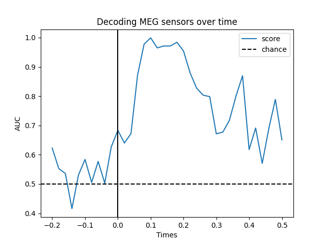
Plot the full (generalization) matrix:

fig, ax = plt.subplots(1, 1)
im = ax.imshow(
    scores,
    interpolation="lanczos",
    origin="lower",
    cmap="RdBu_r",
    extent=epochs.times[[0, -1, 0, -1]],
    vmin=0.0,
    vmax=1.0,
)
ax.set_xlabel("Testing Time (s)")
ax.set_ylabel("Training Time (s)")
ax.set_title("Temporal generalization")
ax.axvline(0, color="k")
ax.axhline(0, color="k")
cbar = plt.colorbar(im, ax=ax)
cbar.set_label("AUC")

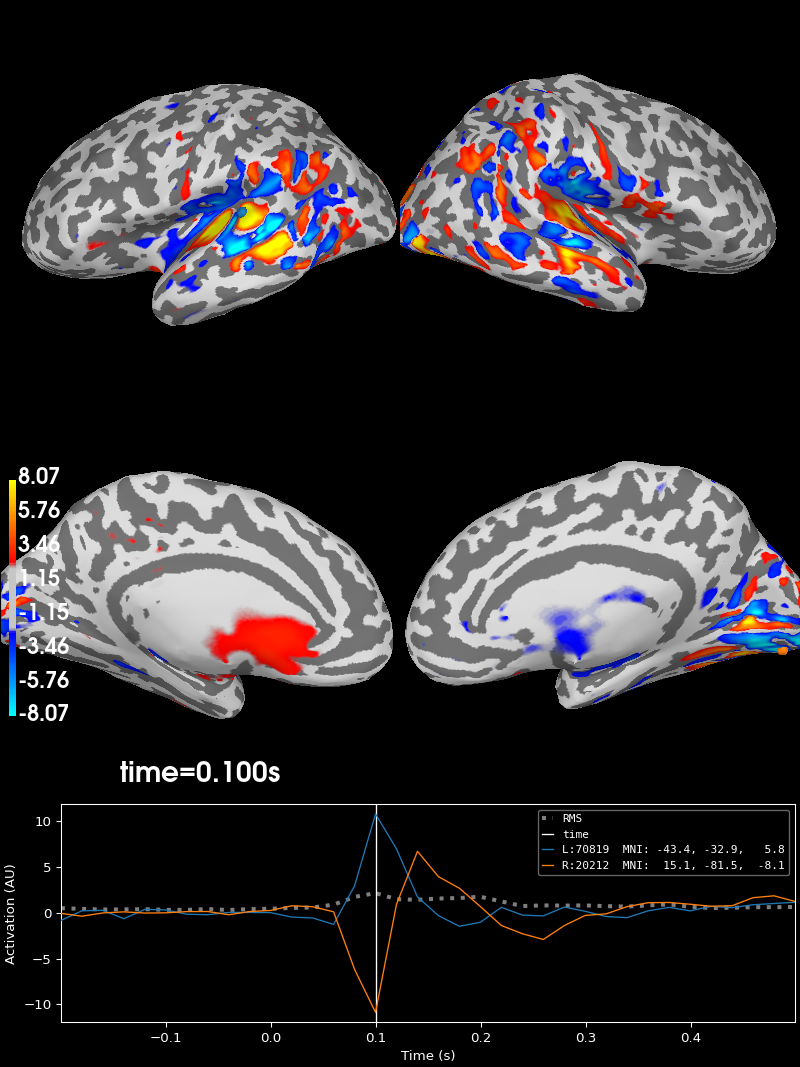
Projecting sensor-space patterns to source space

If you use a linear classifier (or regressor) for your data, you can also project these to source space. For example, using our evoked_time_gen from before:

cov = mne.compute_covariance(epochs, tmax=0.0)
del epochs
fwd = mne.read_forward_solution(meg_path / "sample_audvis-meg-eeg-oct-6-fwd.fif")
inv = mne.minimum_norm.make_inverse_operator(evoked_time_gen.info, fwd, cov, loose=0.0)
stc = mne.minimum_norm.apply_inverse(evoked_time_gen, inv, 1.0 / 9.0, "dSPM")
del fwd, inv

Reducing data rank from 203 -> 203
Estimating covariance using EMPIRICAL
Done.
Number of samples used : 1353
[done]
Reading forward solution from /home/circleci/mne_data/MNE-sample-data/MEG/sample/sample_audvis-meg-eeg-oct-6-fwd.fif...
    Reading a source space...
    Computing patch statistics...
    Patch information added...
    Distance information added...
    [done]
    Reading a source space...
    Computing patch statistics...
    Patch information added...
    Distance information added...
    [done]
    2 source spaces read
    Desired named matrix (kind = 3523 (FIFF_MNE_FORWARD_SOLUTION_GRAD)) not available
    Read MEG forward solution (7498 sources, 306 channels, free orientations)
    Desired named matrix (kind = 3523 (FIFF_MNE_FORWARD_SOLUTION_GRAD)) not available
    Read EEG forward solution (7498 sources, 60 channels, free orientations)
    Forward solutions combined: MEG, EEG
    Source spaces transformed to the forward solution coordinate frame
Computing inverse operator with 203 channels.
    203 out of 366 channels remain after picking
Selected 203 channels
Creating the depth weighting matrix...
    203 planar channels
    limit = 7262/7498 = 10.020866
    scale = 2.58122e-08 exp = 0.8
    Picked elements from a free-orientation depth-weighting prior into the fixed-orientation one
    Average patch normals will be employed in the rotation to the local surface coordinates....
    Converting to surface-based source orientations...
    [done]
Whitening the forward solution.
Computing rank from covariance with rank=None
    Using tolerance 1.6e-13 (2.2e-16 eps * 203 dim * 3.6  max singular value)
    Estimated rank (grad): 203
    GRAD: rank 203 computed from 203 data channels with 0 projectors
    Setting small GRAD eigenvalues to zero (without PCA)
Creating the source covariance matrix
Adjusting source covariance matrix.
Computing SVD of whitened and weighted lead field matrix.
    largest singular value = 3.91709
    scaling factor to adjust the trace = 6.26373e+18 (nchan = 203 nzero = 0)
Preparing the inverse operator for use...
    Scaled noise and source covariance from nave = 1 to nave = 1
    Created the regularized inverter
    The projection vectors do not apply to these channels.
    Created the whitener using a noise covariance matrix with rank 203 (0 small eigenvalues omitted)
    Computing noise-normalization factors (dSPM)...
[done]
Applying inverse operator to ""...
    Picked 203 channels from the data
    Computing inverse...
    Eigenleads need to be weighted ...
    Computing residual...
    Explained  76.4% variance
    dSPM...
[done]

And this can be visualized using stc.plot:

brain = stc.plot(
    hemi="split", views=("lat", "med"), initial_time=0.1, subjects_dir=subjects_dir
)

Using control points [1.98776221 2.41838256 8.06628583]

Source-space decoding

Source space decoding is also possible, but because the number of features can be much larger than in the sensor space, univariate feature selection using ANOVA f-test (or some other metric) can be done to reduce the feature dimension. Interpreting decoding results might be easier in source space as compared to sensor space.

Examples

• Decoding source space data

Exercise

• Explore other datasets from MNE (e.g. Face dataset from SPM to predict Face vs. Scrambled)

References

[1]

Jean-Rémi King, Laura Gwilliams, Chris Holdgraf, Jona Sassenhagen, Alexandre Barachant, Denis Engemann, Eric Larson, and Alexandre Gramfort. Encoding and decoding neuronal dynamics: methodological framework to uncover the algorithms of cognition. hal-01848442, 2018. URL: https://hal.archives-ouvertes.fr/hal-01848442.

[2]

Zoltan J. Koles. The quantitative extraction and topographic mapping of the abnormal components in the clinical EEG. Electroencephalography and Clinical Neurophysiology, 79(6):440–447, 1991. doi:10.1016/0013-4694(91)90163-X.

[3]

Sven Dähne, Frank C. Meinecke, Stefan Haufe, Johannes Höhne, Michael Tangermann, Klaus-Robert Müller, and Vadim V. Nikulin. SPoC: a novel framework for relating the amplitude of neuronal oscillations to behaviorally relevant parameters. NeuroImage, 86:111–122, 2014. doi:10.1016/j.neuroimage.2013.07.079.

[4]

Bertrand Rivet, Antoine Souloumiac, Virginie Attina, and Guillaume Gibert. xDAWN algorithm to enhance evoked potentials: application to brain–computer interface. IEEE Transactions on Biomedical Engineering, 56(8):2035–2043, 2009. doi:10.1109/TBME.2009.2012869.

[5]

Aaron Schurger, Sebastien Marti, and Stanislas Dehaene. Reducing multi-sensor data to a single time course that reveals experimental effects. BMC Neuroscience, 2013. doi:10.1186/1471-2202-14-122.

[6]

Jean-Rémi King, Alexandre Gramfort, Aaron Schurger, Lionel Naccache, and Stanislas Dehaene. Two distinct dynamic modes subtend the detection of unexpected sounds. PLoS ONE, 9(1):e85791, 2014. doi:10.1371/journal.pone.0085791.

[7]

Jean-Rémi King and Stanislas Dehaene. Characterizing the dynamics of mental representations: the temporal generalization method. Trends in Cognitive Sciences, 18(4):203–210, 2014. doi:10.1016/j.tics.2014.01.002.