Linear classifier on sensor data with plot patterns and filters

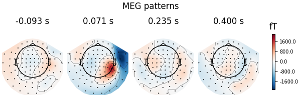
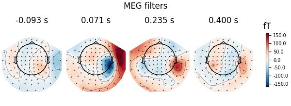
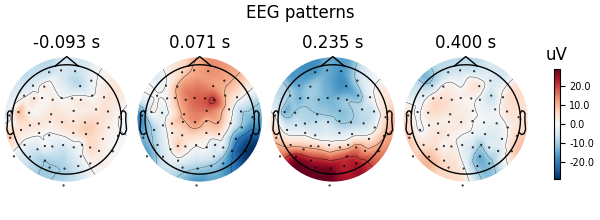
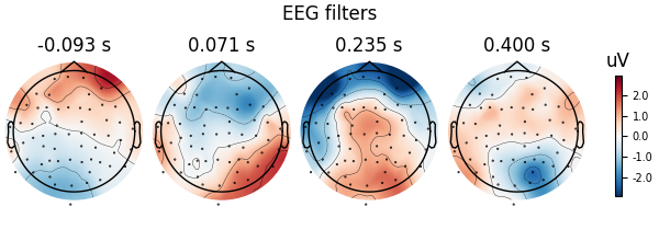
Here decoding, a.k.a MVPA or supervised machine learning, is applied to M/EEG data in sensor space. Fit a linear classifier with the LinearModel object providing topographical patterns which are more neurophysiologically interpretable [1] than the classifier filters (weight vectors). The patterns explain how the MEG and EEG data were generated from the discriminant neural sources which are extracted by the filters. Note patterns/filters in MEG data are more similar than EEG data because the noise is less spatially correlated in MEG than EEG.

# Authors: Alexandre Gramfort <alexandre.gramfort@inria.fr>
#          Romain Trachel <trachelr@gmail.com>
#          Jean-Rémi King <jeanremi.king@gmail.com>
#
# License: BSD-3-Clause
# Copyright the MNE-Python contributors.

from sklearn.linear_model import LogisticRegression
from sklearn.pipeline import make_pipeline
from sklearn.preprocessing import StandardScaler

import mne
from mne import io
from mne.datasets import sample

# import a linear classifier from mne.decoding
from mne.decoding import (
    LinearModel,
    SpatialFilter,
    Vectorizer,
    get_spatial_filter_from_estimator,
)

print(__doc__)

data_path = sample.data_path()
sample_path = data_path / "MEG" / "sample"

Set parameters

raw_fname = sample_path / "sample_audvis_filt-0-40_raw.fif"
event_fname = sample_path / "sample_audvis_filt-0-40_raw-eve.fif"
tmin, tmax = -0.1, 0.4
event_id = dict(aud_l=1, vis_l=3)

# Setup for reading the raw data
raw = io.read_raw_fif(raw_fname, preload=True)
raw.filter(0.5, 25, fir_design="firwin")
events = mne.read_events(event_fname)

# Read epochs
epochs = mne.Epochs(
    raw, events, event_id, tmin, tmax, proj=True, decim=2, baseline=None, preload=True
)
del raw

labels = epochs.events[:, -1]

# get MEG data
meg_epochs = epochs.copy().pick(picks="meg", exclude="bads")
meg_data = meg_epochs.get_data(copy=False).reshape(len(labels), -1)

Opening raw data file /home/circleci/mne_data/MNE-sample-data/MEG/sample/sample_audvis_filt-0-40_raw.fif...
    Read a total of 4 projection items:
        PCA-v1 (1 x 102)  idle
        PCA-v2 (1 x 102)  idle
        PCA-v3 (1 x 102)  idle
        Average EEG reference (1 x 60)  idle
    Range : 6450 ... 48149 =     42.956 ...   320.665 secs
Ready.
Reading 0 ... 41699  =      0.000 ...   277.709 secs...
Filtering raw data in 1 contiguous segment
Setting up band-pass filter from 0.5 - 25 Hz

FIR filter parameters
---------------------
Designing a one-pass, zero-phase, non-causal bandpass filter:
- Windowed time-domain design (firwin) method
- Hamming window with 0.0194 passband ripple and 53 dB stopband attenuation
- Lower passband edge: 0.50
- Lower transition bandwidth: 0.50 Hz (-6 dB cutoff frequency: 0.25 Hz)
- Upper passband edge: 25.00 Hz
- Upper transition bandwidth: 6.25 Hz (-6 dB cutoff frequency: 28.12 Hz)
- Filter length: 993 samples (6.613 s)

Not setting metadata
145 matching events found
No baseline correction applied
Created an SSP operator (subspace dimension = 4)
4 projection items activated
Using data from preloaded Raw for 145 events and 76 original time points (prior to decimation) ...
0 bad epochs dropped

Decoding in sensor space using a LogisticRegression classifier

clf = LogisticRegression(solver="liblinear")  # liblinear is faster than lbfgs
scaler = StandardScaler()

# create a linear model with LogisticRegression
model = LinearModel(clf)

# fit the classifier on MEG data
X = scaler.fit_transform(meg_data)
model.fit(X, labels)

coefs = dict()
for name, coef in (("patterns", model.patterns_), ("filters", model.filters_)):
    # We fit the linear model on Z-scored data. To make the filters
    # interpretable, we must reverse this normalization step
    coef = scaler.inverse_transform([coef])[0]

    # The data was vectorized to fit a single model across all time points and
    # all channels. We thus reshape it:
    coefs[name] = coef.reshape(len(meg_epochs.ch_names), -1).T

# Now we can instantiate the visualization container
spf = SpatialFilter(info=meg_epochs.info, **coefs)
fig = spf.plot_patterns(
    # we will automatically select patterns
    components="auto",
    # as our filters and patterns correspond to actual times
    # we can align them
    tmin=epochs.tmin,
    units="fT",  # it's physical - we inversed the scaling
    show=False,  # to set the title below
    name_format=None,  # to plot actual times
)
fig.suptitle("MEG patterns")
# Same for filters
fig = spf.plot_filters(
    components="auto",
    tmin=epochs.tmin,
    units="fT",
    show=False,
    name_format=None,
)
fig.suptitle("MEG filters")

• 
• 

Let’s do the same on EEG data using a scikit-learn pipeline

X = epochs.pick(picks="eeg", exclude="bads")
y = epochs.events[:, 2]

# Define a unique pipeline to sequentially:
clf = make_pipeline(
    Vectorizer(),  # 1) vectorize across time and channels
    StandardScaler(),  # 2) normalize features across trials
    LinearModel(  # 3) fits a logistic regression
        LogisticRegression(solver="liblinear")
    ),
)
clf.fit(X, y)
spf = get_spatial_filter_from_estimator(
    clf, info=epochs.info, inverse_transform=True, step_name="linearmodel"
)
fig = spf.plot_patterns(
    components="auto",
    tmin=epochs.tmin,
    units="uV",
    show=False,
    name_format=None,
)
fig.suptitle("EEG patterns")
# Same for filters
fig = spf.plot_filters(
    components="auto",
    tmin=epochs.tmin,
    units="uV",
    show=False,
    name_format=None,
)
fig.suptitle("EEG filters")

• 
• 

References

[1]

Stefan Haufe, Frank Meinecke, Kai Görgen, Sven Dähne, John-Dylan Haynes, Benjamin Blankertz, and Felix Bießmann. On the interpretation of weight vectors of linear models in multivariate neuroimaging. NeuroImage, 87:96–110, 2014. doi:10.1016/j.neuroimage.2013.10.067.