Note
Go to the end to download the full example code.
Preprocessing optically pumped magnetometer (OPM) MEG data#
This tutorial covers preprocessing steps that are specific to OPM MEG data. OPMs use a different sensing technology than traditional SQUID MEG systems, which leads to several important differences for analysis:
They are sensitive to DC magnetic fields
Sensor layouts can vary by participant and recording session due to flexible sensor placement
Devices are typically not fixed in place, so the position of the sensors relative to the room (and through the DC fields) can change over time
We will cover some of these considerations here by processing the UCL OPM auditory dataset [1]
# Authors: The MNE-Python contributors.
# License: BSD-3-Clause
# Copyright the MNE-Python contributors.
import matplotlib.pyplot as plt
import nibabel as nib
import numpy as np

import mne

subject = "sub-002"
data_path = mne.datasets.ucl_opm_auditory.data_path()
opm_file = (
    data_path / subject / "ses-001" / "meg" / "sub-002_ses-001_task-aef_run-001_meg.bin"
)
subjects_dir = data_path / "derivatives" / "freesurfer" / "subjects"

# For now we are going to assume the device and head coordinate frames are
# identical (even though this is incorrect), so we pass verbose='error'
raw = mne.io.read_raw_fil(opm_file, verbose="error")
raw.crop(120, 210).load_data()  # crop for speed
Reading 0 ... 540000 = 0.000 ... 90.000 secs...
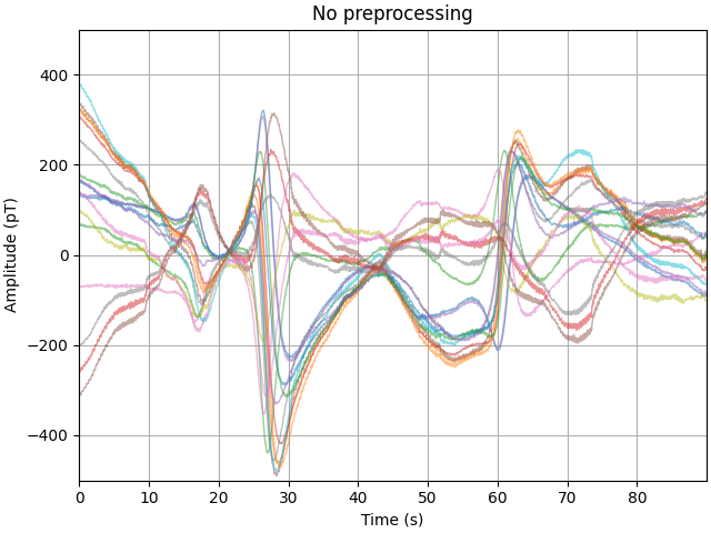
Examining raw data#
First, let’s look at the raw data, noting that there are large fluctuations in the sub 1 Hz band. In some cases the range of fields a single channel reports is as much as 600 pT across this experiment.
picks = mne.pick_types(raw.info, meg=True)

amp_scale = 1e12  # T->pT
stop = len(raw.times) - 300
step = 300
data_ds, time_ds = raw[picks[::5], :stop]
data_ds, time_ds = data_ds[:, ::step] * amp_scale, time_ds[::step]

fig, ax = plt.subplots(layout="constrained")
plot_kwargs = dict(lw=1, alpha=0.5)
ax.plot(time_ds, data_ds.T - np.mean(data_ds, axis=1), **plot_kwargs)
ax.grid(True)
set_kwargs = dict(
    ylim=(-500, 500), xlim=time_ds[[0, -1]], xlabel="Time (s)", ylabel="Amplitude (pT)"
)
ax.set(title="No preprocessing", **set_kwargs)
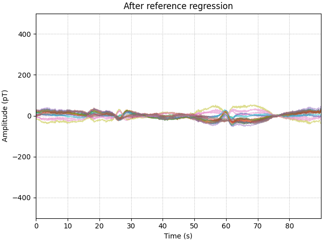
Denoising: Regressing via reference sensors#
The simplest method for reducing low frequency drift in the data is to use a set of reference sensors away from the scalp, which only sample the ambient fields in the room. An advantage of this method is that no prior knowldge of the locations of the sensors is required. However, it assumes that the reference sensors experience the same interference as scalp recordings.
To do this in our current dataset, we require a bit of housekeeping. There are a set of channels beginning with the name “Flux” which do not contain any evironmental data, these need to be set to as bad channels. Another channel – G2-17-TAN – will also be set to bad.
For now we are only interested in removing artefacts seen below 5 Hz, so we initially low-pass filter the good reference channels in this dataset prior to regression
Looking at the processed data, we see there has been a large reduction in the low frequency drift, but there are still periods where the drift has not been entirely removed. The likely cause of this is that the spatial profile of the interference is dynamic, so performing a single regression over the entire experiment is not the most effective approach.
# set flux channels to bad
bad_picks = mne.pick_channels_regexp(raw.ch_names, regexp="Flux.")
raw.info["bads"].extend([raw.ch_names[ii] for ii in bad_picks])
raw.info["bads"].extend(["G2-17-TAN"])

# compute the PSD for later using 1 Hz resolution
psd_kwargs = dict(fmax=20, n_fft=int(round(raw.info["sfreq"])))
psd_pre = raw.compute_psd(**psd_kwargs)

# filter and regress
raw.filter(None, 5, picks="ref_meg")
regress = mne.preprocessing.EOGRegression(picks, picks_artifact="ref_meg")
regress.fit(raw)
regress.apply(raw, copy=False)

# plot
data_ds, _ = raw[picks[::5], :stop]
data_ds = data_ds[:, ::step] * amp_scale

fig, ax = plt.subplots(layout="constrained")
ax.plot(time_ds, data_ds.T - np.mean(data_ds, axis=1), **plot_kwargs)
ax.grid(True, ls=":")
ax.set(title="After reference regression", **set_kwargs)

# compute the psd of the regressed data
psd_post_reg = raw.compute_psd(**psd_kwargs)
Effective window size : 1.000 (s)
Filtering a subset of channels. The highpass and lowpass values in the measurement info will not be updated.
Filtering raw data in 1 contiguous segment
Setting up low-pass filter at 5 Hz

FIR filter parameters
---------------------
Designing a one-pass, zero-phase, non-causal lowpass filter:
- Windowed time-domain design (firwin) method
- Hamming window with 0.0194 passband ripple and 53 dB stopband attenuation
- Upper passband edge: 5.00 Hz
- Upper transition bandwidth: 2.00 Hz (-6 dB cutoff frequency: 6.00 Hz)
- Filter length: 9901 samples (1.650 s)

No projector specified for this dataset. Please consider the method self.add_proj.
No projector specified for this dataset. Please consider the method self.add_proj.
Effective window size : 1.000 (s)
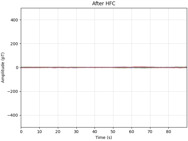
Denoising: Regressing via homogeneous field correction#
Regression of a reference channel is a start, but in this instance assumes the relatiship between the references and a given sensor on the head as constant. However this becomes less accurate when the reference is not moving but the subject is. An alternative method, Homogeneous Field Correction (HFC) only requires that the sensors on the helmet stationary relative to each other. Which in a well-designed rigid helmet is the case.
# include gradients by setting order to 2, set to 1 for homgenous components
projs = mne.preprocessing.compute_proj_hfc(raw.info, order=2)
raw.add_proj(projs).apply_proj(verbose="error")

# plot
data_ds, _ = raw[picks[::5], :stop]
data_ds = data_ds[:, ::step] * amp_scale

fig, ax = plt.subplots(layout="constrained")
ax.plot(time_ds, data_ds.T - np.mean(data_ds, axis=1), **plot_kwargs)
ax.grid(True, ls=":")
ax.set(title="After HFC", **set_kwargs)

# compute the psd of the regressed data
psd_post_hfc = raw.compute_psd(**psd_kwargs)
8 projection items deactivated
Effective window size : 1.000 (s)
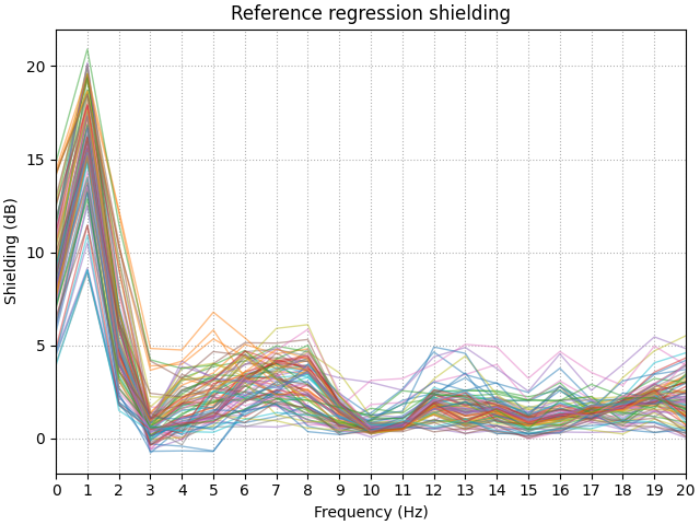
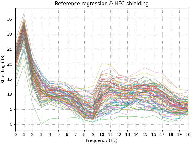
Comparing denoising methods#
Differing denoising methods will have differing levels of performance across different parts of the spectrum. One way to evaluate the performance of a denoising step is to calculate the power spectrum of the dataset before and after processing. We will use metric called the shielding factor to summarise the values. Positive shielding factors indicate a reduction in power, whilst negative means in increase.
We see that reference regression does a good job in reducing low frequency drift up to ~2 Hz, with 20 dB of shielding. But rapidly drops off due to low pass filtering the reference signal at 5 Hz. We also can see that this method is also introducing additional interference at 3 Hz.
HFC improves on the low frequency shielding (up to 32 dB). Also this method is not frequency-specific so we observe broadband interference reduction.
shielding = 10 * np.log10(psd_pre[:] / psd_post_reg[:])

fig, ax = plt.subplots(layout="constrained")
ax.plot(psd_post_reg.freqs, shielding.T, **plot_kwargs)
ax.grid(True, ls=":")
ax.set(xticks=psd_post_reg.freqs)
ax.set(
    xlim=(0, 20),
    title="Reference regression shielding",
    xlabel="Frequency (Hz)",
    ylabel="Shielding (dB)",
)


shielding = 10 * np.log10(psd_pre[:] / psd_post_hfc[:])

fig, ax = plt.subplots(layout="constrained")
ax.plot(psd_post_hfc.freqs, shielding.T, **plot_kwargs)
ax.grid(True, ls=":")
ax.set(xticks=psd_post_hfc.freqs)
ax.set(
    xlim=(0, 20),
    title="Reference regression & HFC shielding",
    xlabel="Frequency (Hz)",
    ylabel="Shielding (dB)",
)
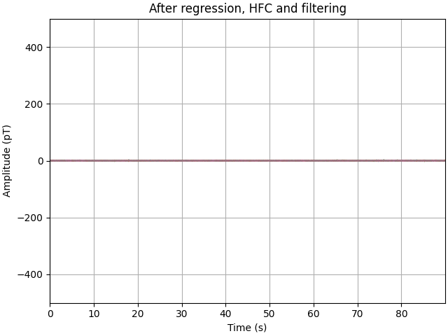
Filtering nuisance signals#
Having regressed much of the high-amplitude, low-frequency interference, we can now look to filtering the remnant nuisance signals. The motivation for filtering after regression (rather than before) is to minimise any filter artefacts generated when removing such high-amplitude interfece (compared to the neural signals we are interested in).
We are going to remove the 50 Hz mains signal with a notch filter, followed by a bandpass filter between 2 and 40 Hz. From here it becomes clear that the variance in our signal has been reduced from 100s of pT to 10s of pT instead.
# notch
raw.notch_filter(np.arange(50, 251, 50), notch_widths=4)
# bandpass
raw.filter(2, 40, picks="meg")
# plot
data_ds, _ = raw[picks[::5], :stop]
data_ds = data_ds[:, ::step] * amp_scale
fig, ax = plt.subplots(layout="constrained")
plot_kwargs = dict(lw=1, alpha=0.5)
ax.plot(time_ds, data_ds.T - np.mean(data_ds, axis=1), **plot_kwargs)
ax.grid(True)
set_kwargs = dict(
    ylim=(-500, 500), xlim=time_ds[[0, -1]], xlabel="Time (s)", ylabel="Amplitude (pT)"
)
ax.set(title="After regression, HFC and filtering", **set_kwargs)
Filtering raw data in 1 contiguous segment
Setting up band-stop filter

FIR filter parameters
---------------------
Designing a one-pass, zero-phase, non-causal bandstop filter:
- Windowed time-domain design (firwin) method
- Hamming window with 0.0194 passband ripple and 53 dB stopband attenuation
- Lower transition bandwidth: 0.50 Hz
- Upper transition bandwidth: 0.50 Hz
- Filter length: 39601 samples (6.600 s)

Filtering a subset of channels. The highpass and lowpass values in the measurement info will not be updated.
Filtering raw data in 1 contiguous segment
Setting up band-pass filter from 2 - 40 Hz

FIR filter parameters
---------------------
Designing a one-pass, zero-phase, non-causal bandpass filter:
- Windowed time-domain design (firwin) method
- Hamming window with 0.0194 passband ripple and 53 dB stopband attenuation
- Lower passband edge: 2.00
- Lower transition bandwidth: 2.00 Hz (-6 dB cutoff frequency: 1.00 Hz)
- Upper passband edge: 40.00 Hz
- Upper transition bandwidth: 10.00 Hz (-6 dB cutoff frequency: 45.00 Hz)
- Filter length: 9901 samples (1.650 s)
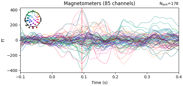
Generating an evoked response#
With the data preprocessed, it is now possible to see an auditory evoked response at the sensor level.
events = mne.find_events(raw, min_duration=0.1)
epochs = mne.Epochs(
    raw, events, tmin=-0.1, tmax=0.4, baseline=(-0.1, 0.0), verbose="error"
)
evoked = epochs.average()
t_peak = evoked.times[np.argmax(np.std(evoked.copy().pick("meg").data, axis=0))]
fig = evoked.plot_joint(picks="mag")
Finding events on: NI-TRIG
180 events found on stim channel NI-TRIG
Event IDs: [3]
Projections have already been applied. Setting proj attribute to True.
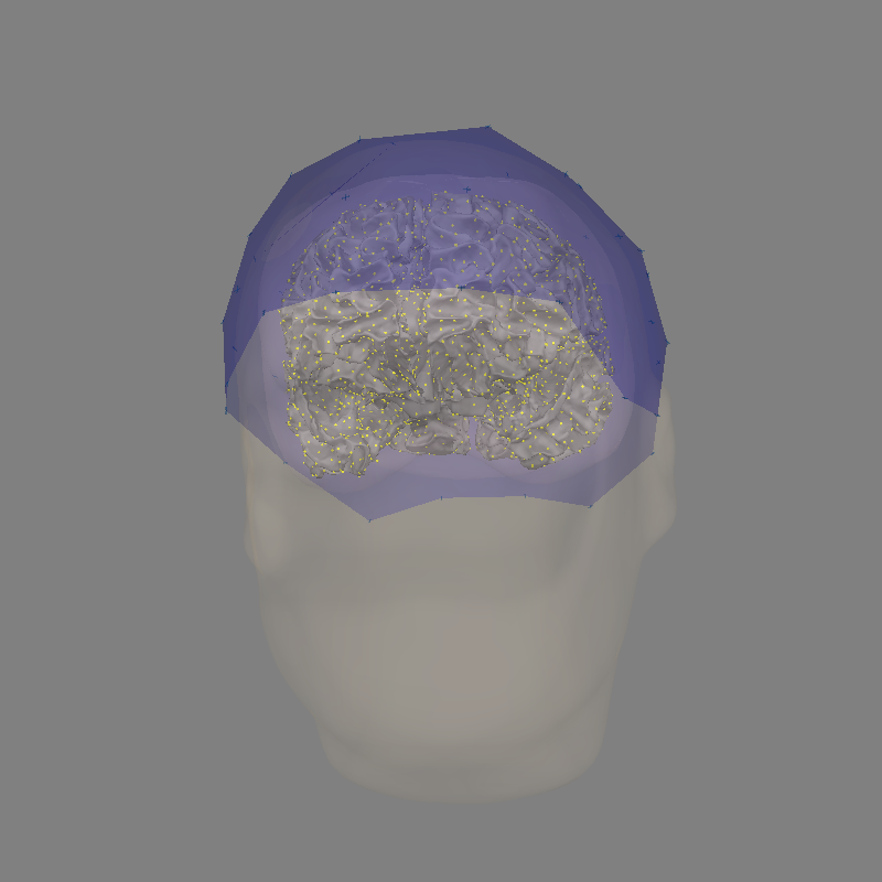
Visualizing coregistration#
By design, the sensors in this dataset are already in the scanner RAS coordinate frame. We can thus visualize them in the FreeSurfer MRI coordinate frame by computing the transformation between the FreeSurfer MRI coordinate frame and scanner RAS:
mri = nib.load(subjects_dir / "sub-002" / "mri" / "T1.mgz")
trans = mri.header.get_vox2ras_tkr() @ np.linalg.inv(mri.affine)
trans[:3, 3] /= 1000.0  # nibabel uses mm, MNE uses m
trans = mne.transforms.Transform("head", "mri", trans)

bem = subjects_dir / subject / "bem" / f"{subject}-5120-bem-sol.fif"
src = subjects_dir / subject / "bem" / f"{subject}-oct-6-src.fif"
mne.viz.plot_alignment(
    evoked.info,
    subjects_dir=subjects_dir,
    subject=subject,
    trans=trans,
    surfaces={"head": 0.1, "inner_skull": 0.2, "white": 1.0},
    meg=["helmet", "sensors"],
    verbose="error",
    bem=bem,
    src=src,
)
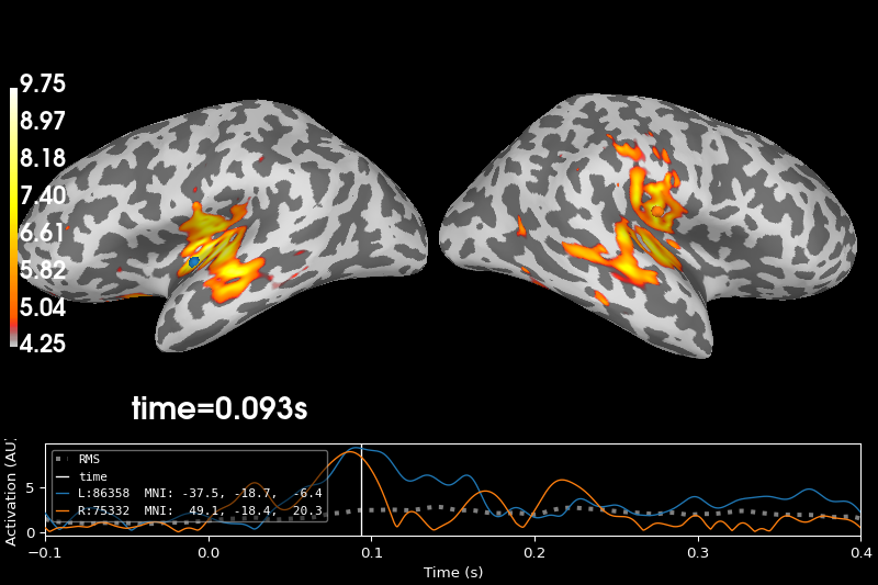
Plotting the inverse#
Now we can compute a forward and inverse:
fwd = mne.make_forward_solution(
    evoked.info,
    trans=trans,
    bem=bem,
    src=src,
    verbose=True,
)
noise_cov = mne.compute_covariance(epochs, tmax=0)
inv = mne.minimum_norm.make_inverse_operator(evoked.info, fwd, noise_cov, verbose=True)
stc = mne.minimum_norm.apply_inverse(
    evoked, inv, 1.0 / 9.0, method="dSPM", verbose=True
)
brain = stc.plot(
    hemi="split",
    size=(800, 400),
    initial_time=t_peak,
    subjects_dir=subjects_dir,
)
Source space          : /home/circleci/mne_data/auditory_OPM_stationary/derivatives/freesurfer/subjects/sub-002/bem/sub-002-oct-6-src.fif
MRI -> head transform : instance of Transform
Measurement data      : instance of Info
Conductor model   : /home/circleci/mne_data/auditory_OPM_stationary/derivatives/freesurfer/subjects/sub-002/bem/sub-002-5120-bem-sol.fif
Accurate field computations
Do computations in head coordinates
Free source orientations

Reading /home/circleci/mne_data/auditory_OPM_stationary/derivatives/freesurfer/subjects/sub-002/bem/sub-002-oct-6-src.fif...
Read 2 source spaces a total of 8196 active source locations

Coordinate transformation: MRI (surface RAS) -> head
    1.000000 0.000000 0.000000       0.50 mm
    0.000000 1.000000 0.000000      26.98 mm
    0.000000 0.000000 1.000000      -9.21 mm
    0.000000 0.000000 0.000000       1.00

Read 94 MEG channels from info
Read 8 MEG compensation channels from info
0 compensation data sets in info
Setting up compensation data...
    No compensation set. Nothing more to do.
105 coil definitions read
Coordinate transformation: MEG device -> head
    1.000000 0.000000 0.000000       0.00 mm
    0.000000 1.000000 0.000000       0.00 mm
    0.000000 0.000000 1.000000       0.00 mm
    0.000000 0.000000 0.000000       1.00
MEG coil definitions created in head coordinates.
Source spaces are now in head coordinates.

Setting up the BEM model using /home/circleci/mne_data/auditory_OPM_stationary/derivatives/freesurfer/subjects/sub-002/bem/sub-002-5120-bem-sol.fif...

Loading surfaces...

Loading the solution matrix...

Homogeneous model surface loaded.
Loaded linear collocation BEM solution from /home/circleci/mne_data/auditory_OPM_stationary/derivatives/freesurfer/subjects/sub-002/bem/sub-002-5120-bem-sol.fif
Employing the head->MRI coordinate transform with the BEM model.
BEM model sub-002-5120-bem-sol.fif is now set up


Source spaces are in head coordinates.
Checking that the sources are inside the surface (will take a few...)
Checking surface interior status for 4098 points...
    Found  535/4098 points inside  an interior sphere of radius   35.6 mm
    Found    0/4098 points outside an exterior sphere of radius   98.5 mm
    Found    0/3563 points outside using surface Qhull
    Found    0/3563 points outside using solid angles
    Total 4098/4098 points inside the surface
Interior check completed in 6916.6 ms
Checking surface interior status for 4098 points...
    Found  501/4098 points inside  an interior sphere of radius   35.6 mm
    Found    0/4098 points outside an exterior sphere of radius   98.5 mm
    Found    0/3597 points outside using surface Qhull
    Found    0/3597 points outside using solid angles
    Total 4098/4098 points inside the surface
Interior check completed in 1522.1 ms
Checking surface interior status for 94 points...
    Found  0/94 points inside  an interior sphere of radius   35.6 mm
    Found 30/94 points outside an exterior sphere of radius   98.5 mm
    Found 64/64 points outside using surface Qhull
    Found  0/ 0 points outside using solid angles
    Total 0/94 points inside the surface
Interior check completed in 13.1 ms

Composing the field computation matrix...
Computing MEG at 8196 source locations (free orientations)...

Finished.
Using data from preloaded Raw for 180 events and 3001 original time points ...
2 bad epochs dropped
    Created an SSP operator (subspace dimension = 8)
    Setting small MAG eigenvalues to zero (without PCA)
Reducing data rank from 85 -> 77
Estimating covariance using EMPIRICAL
Done.
Number of samples used : 106978
[done]
Converting forward solution to surface orientation
    Average patch normals will be employed in the rotation to the local surface coordinates....
    Converting to surface-based source orientations...
    [done]
info["bads"] and noise_cov["bads"] do not match, excluding bad channels from both
Computing inverse operator with 85 channels.
    85 out of 86 channels remain after picking
Selected 85 channels
Creating the depth weighting matrix...
    85 magnetometer or axial gradiometer channels
    limit = 7888/8196 = 10.028156
    scale = 1.9787e-10 exp = 0.8
Applying loose dipole orientations to surface source spaces: 0.2
Whitening the forward solution.
    Created an SSP operator (subspace dimension = 8)
Computing rank from covariance with rank=None
    Using tolerance 4.2e-14 (2.2e-16 eps * 85 dim * 2.2  max singular value)
    Estimated rank (mag): 77
    MAG: rank 77 computed from 85 data channels with 8 projectors
    Setting small MAG eigenvalues to zero (without PCA)
Creating the source covariance matrix
Adjusting source covariance matrix.
Computing SVD of whitened and weighted lead field matrix.
    largest singular value = 2.39473
    scaling factor to adjust the trace = 9.52253e+18 (nchan = 85 nzero = 8)
Preparing the inverse operator for use...
    Scaled noise and source covariance from nave = 1 to nave = 178
    Created the regularized inverter
    Created an SSP operator (subspace dimension = 8)
    Created the whitener using a noise covariance matrix with rank 77 (8 small eigenvalues omitted)
    Computing noise-normalization factors (dSPM)...
[done]
Applying inverse operator to "3"...
    Picked 85 channels from the data
    Computing inverse...
    Eigenleads need to be weighted ...
    Computing residual...
    Explained  90.3% variance
    Combining the current components...
    dSPM...
[done]
Using control points [4.25382465 4.85477031 9.75261481]
References#
Total running time of the script: (0 minutes 51.000 seconds)