Reduce EOG artifacts through regression

Reduce artifacts by regressing the EOG channels onto the rest of the channels and then subtracting the EOG signal.

This is a quick example to show the most basic application of the technique. See the tutorial for a more thorough explanation that demonstrates more advanced approaches.

# Author: Marijn van Vliet <w.m.vanvliet@gmail.com>
#
# License: BSD-3-Clause
# Copyright the MNE-Python contributors.

Import packages and load data

We begin as always by importing the necessary Python modules and loading some data, in this case the MNE sample dataset.

from matplotlib import pyplot as plt

import mne
from mne.datasets import sample
from mne.preprocessing import EOGRegression

print(__doc__)

data_path = sample.data_path()
raw_fname = data_path / "MEG" / "sample" / "sample_audvis_filt-0-40_raw.fif"

# Read raw data
raw = mne.io.read_raw_fif(raw_fname, preload=True)
events = mne.find_events(raw, "STI 014")

# Highpass filter to eliminate slow drifts
raw.filter(0.3, None, picks="all")

Opening raw data file /home/circleci/mne_data/MNE-sample-data/MEG/sample/sample_audvis_filt-0-40_raw.fif...
    Read a total of 4 projection items:
        PCA-v1 (1 x 102)  idle
        PCA-v2 (1 x 102)  idle
        PCA-v3 (1 x 102)  idle
        Average EEG reference (1 x 60)  idle
    Range : 6450 ... 48149 =     42.956 ...   320.665 secs
Ready.
Reading 0 ... 41699  =      0.000 ...   277.709 secs...
319 events found on stim channel STI 014
Event IDs: [ 1  2  3  4  5 32]
Filtering raw data in 1 contiguous segment
Setting up high-pass filter at 0.3 Hz

FIR filter parameters
---------------------
Designing a one-pass, zero-phase, non-causal highpass filter:
- Windowed time-domain design (firwin) method
- Hamming window with 0.0194 passband ripple and 53 dB stopband attenuation
- Lower passband edge: 0.30
- Lower transition bandwidth: 0.30 Hz (-6 dB cutoff frequency: 0.15 Hz)
- Filter length: 1653 samples (11.009 s)

[Parallel(n_jobs=1)]: Done  17 tasks      | elapsed:    0.0s
[Parallel(n_jobs=1)]: Done  71 tasks      | elapsed:    0.1s
[Parallel(n_jobs=1)]: Done 161 tasks      | elapsed:    0.3s
[Parallel(n_jobs=1)]: Done 287 tasks      | elapsed:    0.5s

General

Measurement date	December 03, 2002 19:01:10 GMT
Experimenter	Unknown
Participant	Unknown

Channels

Digitized points	146 points
Good channels	203 Gradiometers, 102 Magnetometers, 9 Stimulus, 59 EEG, 1 EOG
Bad channels	MEG 2443, EEG 053
EOG channels	EOG 061
ECG channels	Not available

Data

Sampling frequency	150.15 Hz
Highpass	0.30 Hz
Lowpass	40.00 Hz
Projections	PCA-v1 : off PCA-v2 : off PCA-v3 : off Average EEG reference : off
Filenames	sample_audvis_filt-0-40_raw.fif
Duration	00:04:38 (HH:MM:SS)

Perform regression and remove EOG

# Fit the regression model
weights = EOGRegression().fit(raw)
raw_clean = weights.apply(raw, copy=True)

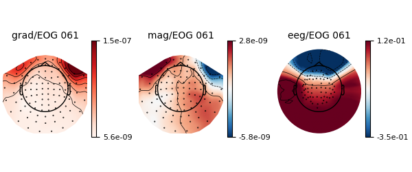
# Show the filter weights in a topomap
weights.plot()

Created an SSP operator (subspace dimension = 4)
4 projection items activated
SSP projectors applied...

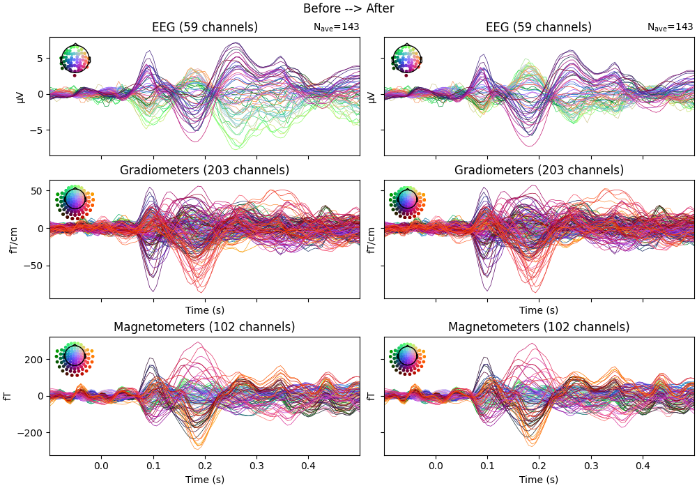
Before/after comparison

Let’s compare the signal before and after cleaning with EOG regression. This is best visualized by extracting epochs and plotting the evoked potential.

tmin, tmax = -0.1, 0.5
event_id = {"visual/left": 3, "visual/right": 4}
evoked_before = mne.Epochs(
    raw, events, event_id, tmin, tmax, baseline=(tmin, 0)
).average()
evoked_after = mne.Epochs(
    raw_clean, events, event_id, tmin, tmax, baseline=(tmin, 0)
).average()

# Create epochs after EOG correction
epochs_after = mne.Epochs(raw_clean, events, event_id, tmin, tmax, baseline=(tmin, 0))
evoked_after = epochs_after.average()

fig, ax = plt.subplots(
    nrows=3, ncols=2, figsize=(10, 7), sharex=True, sharey="row", layout="constrained"
)
evoked_before.plot(axes=ax[:, 0], spatial_colors=True)
evoked_after.plot(axes=ax[:, 1], spatial_colors=True)
fig.suptitle("Before --> After")

Not setting metadata
143 matching events found
Applying baseline correction (mode: mean)
Created an SSP operator (subspace dimension = 4)
4 projection items activated
Not setting metadata
143 matching events found
Applying baseline correction (mode: mean)
Created an SSP operator (subspace dimension = 4)
4 projection items activated
Not setting metadata
143 matching events found
Applying baseline correction (mode: mean)
Created an SSP operator (subspace dimension = 4)
4 projection items activated

Estimated memory usage: 248 MB