Computing a covariance matrix

Many methods in MNE, including source estimation and some classification algorithms, require covariance estimations from the recordings. In this tutorial we cover the basics of sensor covariance computations and construct a noise covariance matrix that can be used when computing the minimum-norm inverse solution. For more information, see The minimum-norm current estimates.

# Authors: The MNE-Python contributors.
# License: BSD-3-Clause
# Copyright the MNE-Python contributors.

import mne
from mne.datasets import sample

Source estimation methods such as MNE require noise estimates from the recordings. In this tutorial we cover the basics of noise covariance and construct a noise covariance matrix that can be used when computing the inverse solution. For more information, see The minimum-norm current estimates.

data_path = sample.data_path()
raw_empty_room_fname = data_path / "MEG" / "sample" / "ernoise_raw.fif"
raw_empty_room = mne.io.read_raw_fif(raw_empty_room_fname)
raw_fname = data_path / "MEG" / "sample" / "sample_audvis_raw.fif"
raw = mne.io.read_raw_fif(raw_fname)
raw.set_eeg_reference("average", projection=True)
raw.info["bads"] += ["EEG 053"]  # bads + 1 more

Opening raw data file /home/circleci/mne_data/MNE-sample-data/MEG/sample/ernoise_raw.fif...
Isotrak not found
    Read a total of 3 projection items:
        PCA-v1 (1 x 102)  idle
        PCA-v2 (1 x 102)  idle
        PCA-v3 (1 x 102)  idle
    Range : 19800 ... 85867 =     32.966 ...   142.965 secs
Ready.
Opening raw data file /home/circleci/mne_data/MNE-sample-data/MEG/sample/sample_audvis_raw.fif...
    Read a total of 3 projection items:
        PCA-v1 (1 x 102)  idle
        PCA-v2 (1 x 102)  idle
        PCA-v3 (1 x 102)  idle
    Range : 25800 ... 192599 =     42.956 ...   320.670 secs
Ready.
EEG channel type selected for re-referencing
Adding average EEG reference projection.
1 projection items deactivated

The definition of noise depends on the paradigm. In MEG it is quite common to use empty room measurements for the estimation of sensor noise. However if you are dealing with evoked responses, you might want to also consider resting state brain activity as noise. First we compute the noise using empty room recording. Note that you can also use only a part of the recording with tmin and tmax arguments. That can be useful if you use resting state as a noise baseline. Here we use the whole empty room recording to compute the noise covariance (tmax=None is the same as the end of the recording, see mne.compute_raw_covariance()).

Keep in mind that you want to match your empty room dataset to your actual MEG data, processing-wise. Ensure that filters are all the same and if you use ICA, apply it to your empty-room and subject data equivalently. In this case we did not filter the data and we don’t use ICA. However, we do have bad channels and projections in the MEG data, and, hence, we want to make sure they get stored in the covariance object.

raw_empty_room.info["bads"] = [bb for bb in raw.info["bads"] if "EEG" not in bb]
raw_empty_room.add_proj(
    [pp.copy() for pp in raw.info["projs"] if "EEG" not in pp["desc"]]
)

noise_cov = mne.compute_raw_covariance(raw_empty_room, tmin=0, tmax=None)

3 projection items deactivated
Using up to 550 segments
Number of samples used : 66000
[done]

Now that you have the covariance matrix in an MNE-Python object you can save it to a file with mne.write_cov(). Later you can read it back using mne.read_cov().

You can also use the pre-stimulus baseline to estimate the noise covariance. First we have to construct the epochs. When computing the covariance, you should use baseline correction when constructing the epochs. Otherwise the covariance matrix will be inaccurate. In MNE this is done by default, but just to be sure, we define it here manually.

events = mne.find_events(raw)
epochs = mne.Epochs(
    raw,
    events,
    event_id=1,
    tmin=-0.2,
    tmax=0.5,
    baseline=(-0.2, 0.0),
    decim=3,  # we'll decimate for speed
    verbose="error",
)  # and ignore the warning about aliasing

320 events found on stim channel STI 014
Event IDs: [ 1  2  3  4  5 32]

Note that this method also attenuates any activity in your source estimates that resemble the baseline, if you like it or not.

noise_cov_baseline = mne.compute_covariance(epochs, tmax=0)

Loading data for 72 events and 421 original time points (prior to decimation) ...
0 bad epochs dropped
    Created an SSP operator (subspace dimension = 4)
    Setting small MEG eigenvalues to zero (without PCA)
    Setting small EEG eigenvalues to zero (without PCA)
Reducing data rank from 364 -> 360
Estimating covariance using EMPIRICAL
Done.
Number of samples used : 2952
[done]

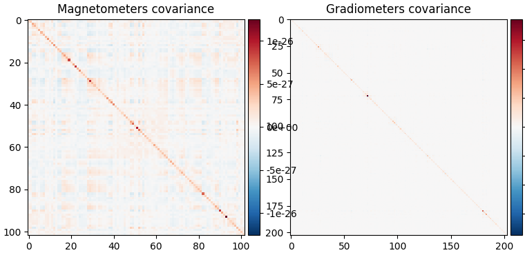
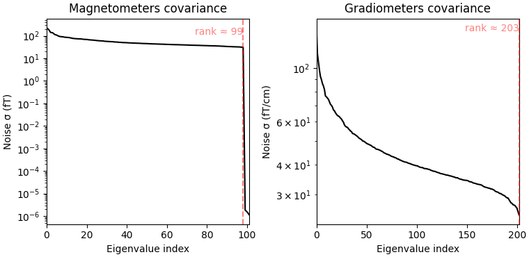
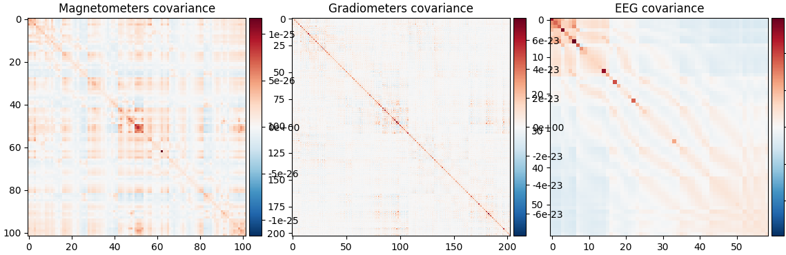
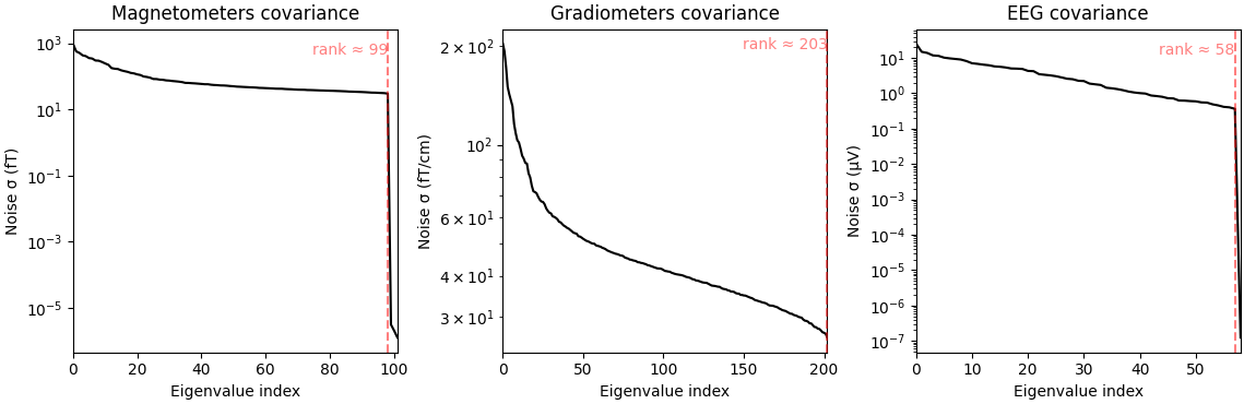
Plot the covariance matrices

Try setting proj to False to see the effect. Notice that the projectors in epochs are already applied, so proj parameter has no effect.

noise_cov.plot(raw_empty_room.info, proj=True)
noise_cov_baseline.plot(epochs.info, proj=True)

• 
• 
• 
• 

    Created an SSP operator (subspace dimension = 3)
Computing rank from covariance with rank=None
    Using tolerance 1.2e-15 (2.2e-16 eps * 102 dim * 0.052  max singular value)
    Estimated rank (mag): 99
    MAG: rank 99 computed from 102 data channels with 0 projectors
Computing rank from covariance with rank=None
    Using tolerance 9.7e-14 (2.2e-16 eps * 203 dim * 2.2  max singular value)
    Estimated rank (grad): 203
    GRAD: rank 203 computed from 203 data channels with 0 projectors
    Created an SSP operator (subspace dimension = 4)
Computing rank from covariance with rank=None
    Using tolerance 2.2e-14 (2.2e-16 eps * 102 dim * 0.96  max singular value)
    Estimated rank (mag): 99
    MAG: rank 99 computed from 102 data channels with 0 projectors
Computing rank from covariance with rank=None
    Using tolerance 1.9e-13 (2.2e-16 eps * 203 dim * 4.1  max singular value)
    Estimated rank (grad): 203
    GRAD: rank 203 computed from 203 data channels with 0 projectors
Computing rank from covariance with rank=None
    Using tolerance 8.4e-14 (2.2e-16 eps * 59 dim * 6.4  max singular value)
    Estimated rank (eeg): 58
    EEG: rank 58 computed from 59 data channels with 0 projectors

How should I regularize the covariance matrix?

The estimated covariance can be numerically unstable and tends to induce correlations between estimated source amplitudes and the number of samples available. The MNE manual therefore suggests to regularize the noise covariance matrix (see Regularization of the noise-covariance matrix), especially if only few samples are available. Unfortunately it is not easy to tell the effective number of samples, hence, to choose the appropriate regularization. In MNE-Python, regularization is done using advanced regularization methods described in Engemann and Gramfort[1]. For this the 'auto' option can be used. With this option, cross-validation will be used to learn the optimal regularization:

noise_cov_reg = mne.compute_covariance(epochs, tmax=0.0, method="auto", rank=None)

Loading data for 72 events and 421 original time points (prior to decimation) ...
    Created an SSP operator (subspace dimension = 4)
    Setting small MEG eigenvalues to zero (without PCA)
    Setting small EEG eigenvalues to zero (without PCA)
Reducing data rank from 364 -> 360
Estimating covariance using SHRUNK
Done.
Estimating covariance using DIAGONAL_FIXED
    MAG regularization : 0.1
    GRAD regularization : 0.1
    EEG regularization : 0.1
Done.
Estimating covariance using EMPIRICAL
Done.
Using cross-validation to select the best estimator.
    MAG regularization : 0.1
    GRAD regularization : 0.1
    EEG regularization : 0.1
    MAG regularization : 0.1
    GRAD regularization : 0.1
    EEG regularization : 0.1
    MAG regularization : 0.1
    GRAD regularization : 0.1
    EEG regularization : 0.1
Number of samples used : 2952
log-likelihood on unseen data (descending order):
   shrunk: -1769.599
   diagonal_fixed: -1785.406
   empirical: -1797.005
selecting best estimator: shrunk
[done]

This procedure evaluates the noise covariance quantitatively by how well it whitens the data using the negative log-likelihood of unseen data. The final result can also be visually inspected. Under the assumption that the baseline does not contain a systematic signal (time-locked to the event of interest), the whitened baseline signal should be follow a multivariate Gaussian distribution, i.e., whitened baseline signals should be between -1.96 and 1.96 at a given time sample. 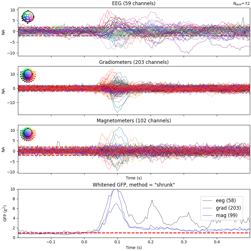Based on the same reasoning, the expected value for the global field power (GFP) is 1 (calculation of the GFP should take into account the true degrees of freedom, e.g. ddof=3 with 2 active SSP vectors):

evoked = epochs.average()
evoked.plot_white(noise_cov_reg, time_unit="s")

NOTE: pick_types() is a legacy function. New code should use inst.pick(...).
Computing rank from covariance with rank=None
    Using tolerance 8.4e-14 (2.2e-16 eps * 59 dim * 6.4  max singular value)
    Estimated rank (eeg): 58
    EEG: rank 58 computed from 59 data channels with 1 projector
Computing rank from covariance with rank=None
    Using tolerance 1.8e-13 (2.2e-16 eps * 203 dim * 4  max singular value)
    Estimated rank (grad): 203
    GRAD: rank 203 computed from 203 data channels with 0 projectors
Computing rank from covariance with rank=None
    Using tolerance 2.1e-14 (2.2e-16 eps * 102 dim * 0.91  max singular value)
    Estimated rank (mag): 99
    MAG: rank 99 computed from 102 data channels with 3 projectors
    Created an SSP operator (subspace dimension = 4)
Computing rank from covariance with rank={'eeg': 58, 'grad': 203, 'mag': 99, 'meg': 302}
    Setting small MEG eigenvalues to zero (without PCA)
    Setting small EEG eigenvalues to zero (without PCA)
    Created the whitener using a noise covariance matrix with rank 360 (4 small eigenvalues omitted)

This plot displays both, the whitened evoked signals for each channels and the whitened GFP. The numbers in the GFP panel represent the estimated rank of the data, which amounts to the effective degrees of freedom by which the squared sum across sensors is divided when computing the whitened GFP. The whitened GFP also helps detecting spurious late evoked components which can be the consequence of over- or under-regularization.

Note that if data have been processed using signal space separation (SSS) [2], gradiometers and magnetometers will be displayed jointly because both are reconstructed from the same SSS basis vectors with the same numerical rank. This also implies that both sensor types are not any longer statistically independent. These methods for evaluation can be used to assess model violations. Additional introductory materials can be found here.

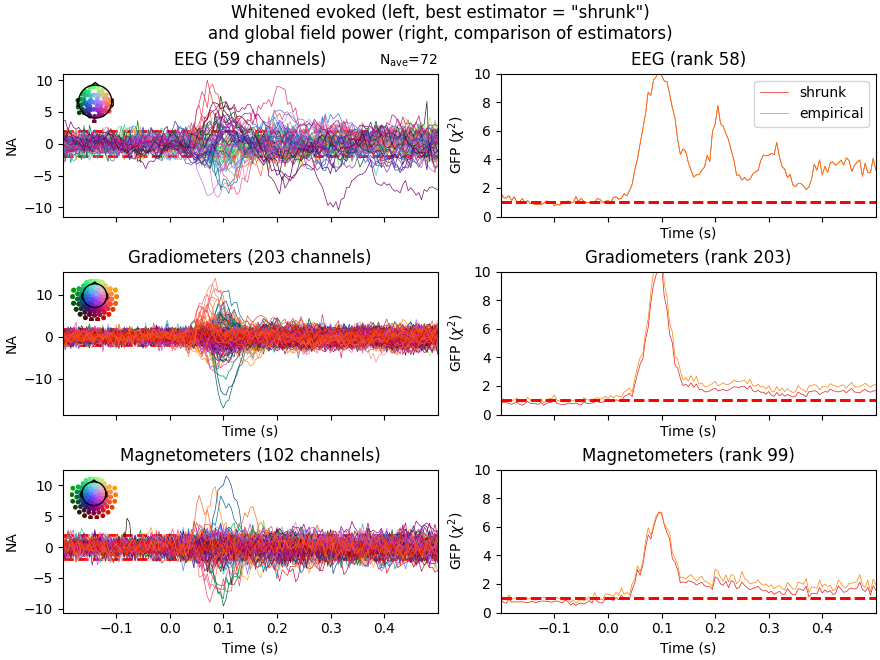
For expert use cases or debugging the alternative estimators can also be compared (see Whitening evoked data with a noise covariance):

noise_covs = mne.compute_covariance(
    epochs, tmax=0.0, method=("empirical", "shrunk"), return_estimators=True, rank=None
)
evoked.plot_white(noise_covs, time_unit="s")

Loading data for 72 events and 421 original time points (prior to decimation) ...
    Created an SSP operator (subspace dimension = 4)
    Setting small MEG eigenvalues to zero (without PCA)
    Setting small EEG eigenvalues to zero (without PCA)
Reducing data rank from 364 -> 360
Estimating covariance using EMPIRICAL
Done.
Estimating covariance using SHRUNK
Done.
Using cross-validation to select the best estimator.
Number of samples used : 2952
log-likelihood on unseen data (descending order):
   shrunk: -1769.599
   empirical: -1797.005
[done]
NOTE: pick_types() is a legacy function. New code should use inst.pick(...).
Computing rank from covariance with rank=None
    Using tolerance 8.4e-14 (2.2e-16 eps * 59 dim * 6.4  max singular value)
    Estimated rank (eeg): 58
    EEG: rank 58 computed from 59 data channels with 1 projector
Computing rank from covariance with rank=None
    Using tolerance 1.8e-13 (2.2e-16 eps * 203 dim * 4  max singular value)
    Estimated rank (grad): 203
    GRAD: rank 203 computed from 203 data channels with 0 projectors
Computing rank from covariance with rank=None
    Using tolerance 2.1e-14 (2.2e-16 eps * 102 dim * 0.91  max singular value)
    Estimated rank (mag): 99
    MAG: rank 99 computed from 102 data channels with 3 projectors
Computing rank from covariance with rank=None
    Using tolerance 8.4e-14 (2.2e-16 eps * 59 dim * 6.4  max singular value)
    Estimated rank (eeg): 58
    EEG: rank 58 computed from 59 data channels with 1 projector
Computing rank from covariance with rank=None
    Using tolerance 1.9e-13 (2.2e-16 eps * 203 dim * 4.1  max singular value)
    Estimated rank (grad): 203
    GRAD: rank 203 computed from 203 data channels with 0 projectors
Computing rank from covariance with rank=None
    Using tolerance 2.2e-14 (2.2e-16 eps * 102 dim * 0.96  max singular value)
    Estimated rank (mag): 99
    MAG: rank 99 computed from 102 data channels with 3 projectors
    Created an SSP operator (subspace dimension = 4)
Computing rank from covariance with rank={'eeg': 58, 'grad': 203, 'mag': 99, 'meg': 302}
    Setting small MEG eigenvalues to zero (without PCA)
    Setting small EEG eigenvalues to zero (without PCA)
    Created the whitener using a noise covariance matrix with rank 360 (4 small eigenvalues omitted)
    Created an SSP operator (subspace dimension = 4)
Computing rank from covariance with rank={'eeg': 58, 'grad': 203, 'mag': 99, 'meg': 302}
    Setting small MEG eigenvalues to zero (without PCA)
    Setting small EEG eigenvalues to zero (without PCA)
    Created the whitener using a noise covariance matrix with rank 360 (4 small eigenvalues omitted)

This will plot the whitened evoked for the optimal estimator and display the GFP for all estimators as separate lines in the related panel.

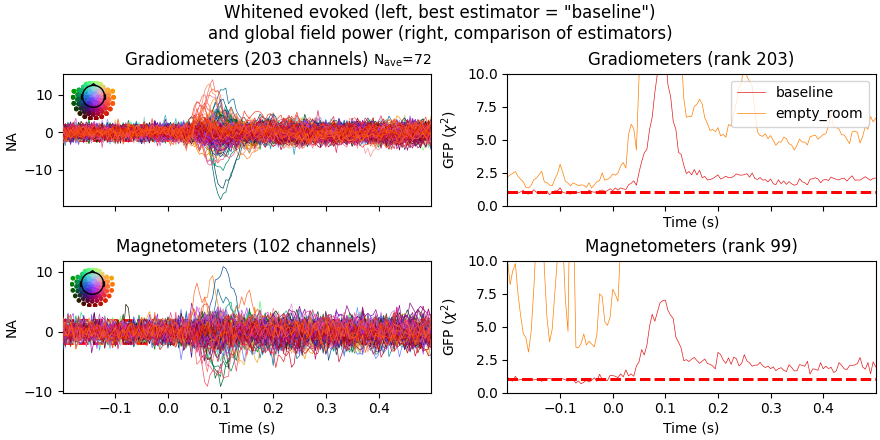
Finally, let’s have a look at the difference between empty room and event related covariance, hacking the "method" option so that their types are shown in the legend of the plot.

evoked_meg = evoked.copy().pick("meg")
noise_cov["method"] = "empty_room"
noise_cov_baseline["method"] = "baseline"
evoked_meg.plot_white([noise_cov_baseline, noise_cov], time_unit="s")

NOTE: pick_types() is a legacy function. New code should use inst.pick(...).
Computing rank from covariance with rank=None
    Using tolerance 1.9e-13 (2.2e-16 eps * 203 dim * 4.1  max singular value)
    Estimated rank (grad): 203
    GRAD: rank 203 computed from 203 data channels with 0 projectors
Computing rank from covariance with rank=None
    Using tolerance 2.2e-14 (2.2e-16 eps * 102 dim * 0.96  max singular value)
    Estimated rank (mag): 99
    MAG: rank 99 computed from 102 data channels with 3 projectors
Computing rank from covariance with rank=None
    Using tolerance 9.7e-14 (2.2e-16 eps * 203 dim * 2.2  max singular value)
    Estimated rank (grad): 203
    GRAD: rank 203 computed from 203 data channels with 0 projectors
Computing rank from covariance with rank=None
    Using tolerance 1.2e-15 (2.2e-16 eps * 102 dim * 0.052  max singular value)
    Estimated rank (mag): 99
    MAG: rank 99 computed from 102 data channels with 3 projectors
    Created an SSP operator (subspace dimension = 3)
Computing rank from covariance with rank={'grad': 203, 'mag': 99, 'meg': 302}
    Setting small MEG eigenvalues to zero (without PCA)
    Created the whitener using a noise covariance matrix with rank 302 (3 small eigenvalues omitted)
    Created an SSP operator (subspace dimension = 3)
Computing rank from covariance with rank={'grad': 203, 'mag': 99, 'meg': 302}
    Setting small MEG eigenvalues to zero (without PCA)
    Created the whitener using a noise covariance matrix with rank 302 (3 small eigenvalues omitted)

Based on the negative log-likelihood, the baseline covariance seems more appropriate. Improper regularization can lead to overestimation of source amplitudes, see [1] for more information and examples.

References

[1] (1,2)

Denis A. Engemann and Alexandre Gramfort. Automated model selection in covariance estimation and spatial whitening of MEG and EEG signals. NeuroImage, 108:328–342, 2015. doi:10.1016/j.neuroimage.2014.12.040.

[2]

Samu Taulu, Juha Simola, and Matti J. Kajola. Applications of the signal space separation method. IEEE Transactions on Signal Processing, 53(9):3359–3372, 2005. doi:10.1109/TSP.2005.853302.