Note
Go to the end to download the full example code.
EEG source localization given electrode locations on an MRI#
This tutorial explains how to compute the forward operator from EEG data when the electrodes are in MRI voxel coordinates.
# Authors: Eric Larson <larson.eric.d@gmail.com>
#
# License: BSD-3-Clause
# Copyright the MNE-Python contributors.
import nibabel
import numpy as np
from nilearn.plotting import plot_glass_brain

import mne
from mne.channels import compute_native_head_t, read_custom_montage
from mne.viz import plot_alignment
Prerequisites#
For this we will assume that you have:
raw EEG data
your subject’s MRI reconstrcted using FreeSurfer
an appropriate boundary element model (BEM)
an appropriate source space (src)
your EEG electrodes in FreeSurfer surface RAS coordinates, stored in one of the formats
mne.channels.read_custom_montage()supports
Let’s set the paths to these files for the sample dataset, including
a modified sample MRI showing the electrode locations plus a .elc
file corresponding to the points in MRI coords (these were synthesized,
and thus are stored as part of the misc dataset).
data_path = mne.datasets.sample.data_path()
subjects_dir = data_path / "subjects"
fname_raw = data_path / "MEG" / "sample" / "sample_audvis_raw.fif"
bem_dir = subjects_dir / "sample" / "bem"
fname_bem = bem_dir / "sample-5120-5120-5120-bem-sol.fif"
fname_src = bem_dir / "sample-oct-6-src.fif"

misc_path = mne.datasets.misc.data_path()
fname_T1_electrodes = misc_path / "sample_eeg_mri" / "T1_electrodes.mgz"
fname_mon = misc_path / "sample_eeg_mri" / "sample_mri_montage.elc"
Visualizing the MRI#
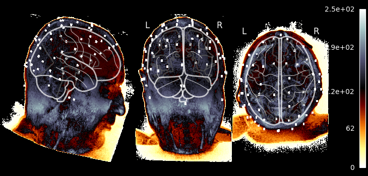
Let’s take our MRI-with-eeg-locations and adjust the affine to put the data
in MNI space, and plot using nilearn.plotting.plot_glass_brain(),
which does a maximum intensity projection (easy to see the fake electrodes).
This plotting function requires data to be in MNI space.
Because img.affine gives the voxel-to-world (RAS) mapping, if we apply a
RAS-to-MNI transform to it, it becomes the voxel-to-MNI transformation we
need. Thus we create a “new” MRI image in MNI coordinates and plot it as:
img = nibabel.load(fname_T1_electrodes)  # original subject MRI w/EEG
ras_mni_t = mne.transforms.read_ras_mni_t("sample", subjects_dir)  # from FS
mni_affine = np.dot(ras_mni_t["trans"], img.affine)  # vox->ras->MNI
img_mni = nibabel.Nifti1Image(img.dataobj, mni_affine)  # now in MNI coords!
plot_glass_brain(
    img_mni,
    cmap="hot_black_bone",
    threshold=0.0,
    black_bg=True,
    resampling_interpolation="nearest",
    colorbar=True,
)
Getting our MRI voxel EEG locations to head (and MRI surface RAS) coords#
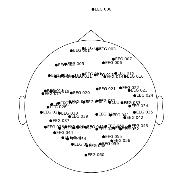
Let’s load our DigMontage using
mne.channels.read_custom_montage(), making note of the fact that
we stored our locations in FreeSurfer surface RAS (MRI) coordinates.
What if my electrodes are in MRI voxels?
If you have voxel coordinates in MRI voxels, you can transform these to
FreeSurfer surface RAS (called “mri” in MNE) coordinates using the
transformations that FreeSurfer computes during reconstruction.
nibabel calls this transformation the vox2ras_tkr transform
and operates in millimeters, so we can load it, convert it to meters,
and then apply it:
You can also verify that these are correct (or manually convert voxels to MRI coords) by looking at the points in Freeview or tkmedit.
dig_montage = read_custom_montage(
fname_mon,
head_size=None,
coord_frame="mri",
verbose="error", # because it contains a duplicate point
)
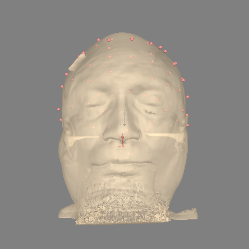
dig_montage.plot()
We can then get our transformation from the MRI coordinate frame (where our points are defined) to the head coordinate frame from the object.
trans = compute_native_head_t(dig_montage)
print(trans)  # should be mri->head, as the "native" space here is MRI
<Transform | MRI (surface RAS)->head>
[[ 0.99930957  0.00998471 -0.03578661 -0.00316747]
 [ 0.01275917  0.81240435  0.58295487  0.00685511]
 [ 0.03489383 -0.58300899  0.81171605  0.02888406]
 [ 0.          0.          0.          1.        ]]
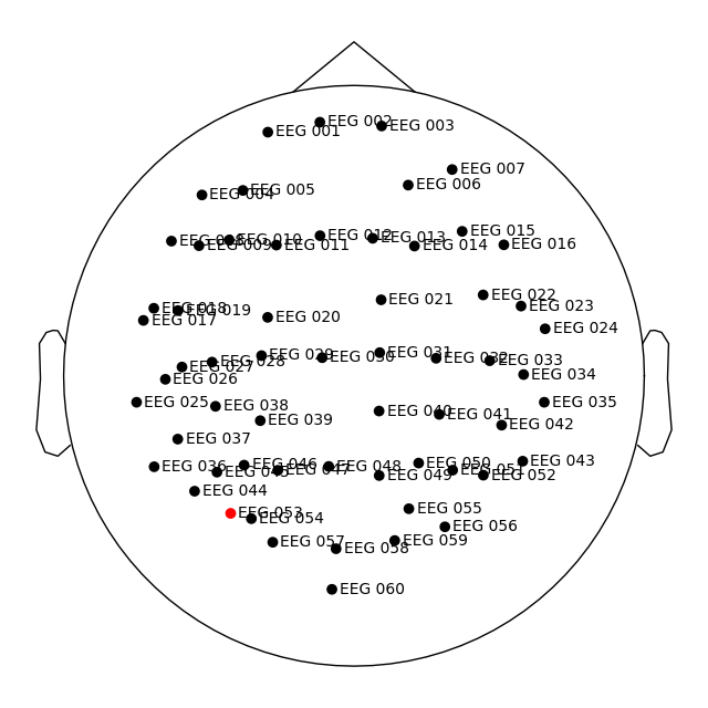
Let’s apply this digitization to our dataset, and in the process
automatically convert our locations to the head coordinate frame, as
shown by plot_sensors().
raw = mne.io.read_raw_fif(fname_raw)
raw.pick(picks=["eeg", "stim"]).load_data()
raw.set_montage(dig_montage)
raw.plot_sensors(show_names=True)
Opening raw data file /home/circleci/mne_data/MNE-sample-data/MEG/sample/sample_audvis_raw.fif...
    Read a total of 3 projection items:
        PCA-v1 (1 x 10²)  idle
        PCA-v2 (1 x 10²)  idle
        PCA-v3 (1 x 10²)  idle
    Range : 25800 ... 192599 =     42.956 ...   320.670 secs
Ready.
Reading 0 ... 166799  =      0.000 ...   277.714 secs...
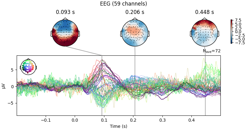
Now we can do standard sensor-space operations like make joint plots of evoked data.
raw.set_eeg_reference(projection=True)
events = mne.find_events(raw)
epochs = mne.Epochs(raw, events)
cov = mne.compute_covariance(epochs, tmax=0.0)
evoked = epochs["1"].average()  # trigger 1 in auditory/left
evoked.plot_joint()
EEG channel type selected for re-referencing
Adding average EEG reference projection.
1 projection items deactivated
Average reference projection was added, but has not been applied yet. Use the apply_proj method to apply it.
Finding events on: STI 014
320 events found on stim channel STI 014
Event IDs: [ 1  2  3  4  5 32]
Not setting metadata
320 matching events found
Setting baseline interval to [-0.19979521315838786, 0.0] s
Applying baseline correction (mode: mean)
Created an SSP operator (subspace dimension = 1)
1 projection items activated
Using data from preloaded Raw for 72 events and 421 original time points ...
0 bad epochs dropped
Using data from preloaded Raw for 73 events and 421 original time points ...
0 bad epochs dropped
Using data from preloaded Raw for 73 events and 421 original time points ...
0 bad epochs dropped
Using data from preloaded Raw for 71 events and 421 original time points ...
0 bad epochs dropped
Using data from preloaded Raw for 15 events and 421 original time points ...
0 bad epochs dropped
Using data from preloaded Raw for 16 events and 421 original time points ...
0 bad epochs dropped
    Created an SSP operator (subspace dimension = 1)
    Setting small EEG eigenvalues to zero (without PCA)
Reducing data rank from 59 -> 58
Estimating covariance using EMPIRICAL
Done.
Number of samples used : 38720
[done]
Projections have already been applied. Setting proj attribute to True.
Getting a source estimate#
New we have all of the components we need to compute a forward solution, but first we should sanity check that everything is well aligned:
fig = plot_alignment(
    evoked.info,
    trans=trans,
    show_axes=True,
    surfaces="head-dense",
    subject="sample",
    subjects_dir=subjects_dir,
)
Using lh.seghead for head surface.
Channel types:: eeg: 59
Now we can actually compute the forward:
fwd = mne.make_forward_solution(
    evoked.info, trans=trans, src=fname_src, bem=fname_bem, verbose=True
)
Source space          : /home/circleci/mne_data/MNE-sample-data/subjects/sample/bem/sample-oct-6-src.fif
MRI -> head transform : instance of Transform
Measurement data      : instance of Info
Conductor model   : /home/circleci/mne_data/MNE-sample-data/subjects/sample/bem/sample-5120-5120-5120-bem-sol.fif
Accurate field computations
Do computations in head coordinates
Free source orientations

Reading /home/circleci/mne_data/MNE-sample-data/subjects/sample/bem/sample-oct-6-src.fif...
Read 2 source spaces a total of 8196 active source locations

Coordinate transformation: MRI (surface RAS) -> head
    0.999310 0.009985 -0.035787      -3.17 mm
    0.012759 0.812404 0.582955       6.86 mm
    0.034894 -0.583009 0.811716      28.88 mm
    0.000000 0.000000 0.000000       1.00

Read  60 EEG channels from info
Head coordinate coil definitions created.
Source spaces are now in head coordinates.

Setting up the BEM model using /home/circleci/mne_data/MNE-sample-data/subjects/sample/bem/sample-5120-5120-5120-bem-sol.fif...

Loading surfaces...

Loading the solution matrix...

Three-layer model surfaces loaded.
Loaded linear collocation BEM solution from /home/circleci/mne_data/MNE-sample-data/subjects/sample/bem/sample-5120-5120-5120-bem-sol.fif
Employing the head->MRI coordinate transform with the BEM model.
BEM model sample-5120-5120-5120-bem-sol.fif is now set up


Source spaces are in head coordinates.
Checking that the sources are inside the surface (will take a few...)
Checking surface interior status for 4098 points...
    Found  846/4098 points inside  an interior sphere of radius   43.6 mm
    Found    0/4098 points outside an exterior sphere of radius   91.8 mm
    Found    2/3252 points outside using surface Qhull
    Found    0/3250 points outside using solid angles
    Total 4096/4098 points inside the surface
Interior check completed in 3559.2 ms
    2 source space points omitted because they are outside the inner skull surface.
    Computing patch statistics...
    Patch information added...
Checking surface interior status for 4098 points...
    Found  875/4098 points inside  an interior sphere of radius   43.6 mm
    Found    0/4098 points outside an exterior sphere of radius   91.8 mm
    Found    0/3223 points outside using surface Qhull
    Found    1/3223 point  outside using solid angles
    Total 4097/4098 points inside the surface
Interior check completed in 4553.6 ms
    1 source space point omitted because it is outside the inner skull surface.
    Computing patch statistics...
    Patch information added...
Setting up for EEG...
Computing EEG at 8193 source locations (free orientations)...

Finished.
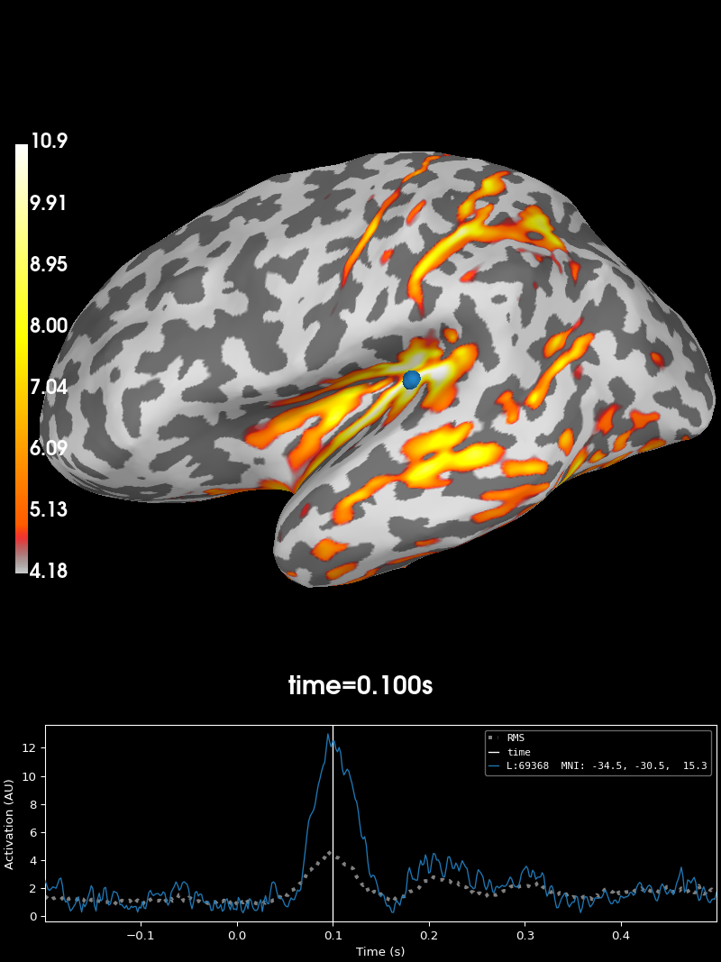
Finally let’s compute the inverse and apply it:
inv = mne.minimum_norm.make_inverse_operator(evoked.info, fwd, cov, verbose=True)
stc = mne.minimum_norm.apply_inverse(evoked, inv)
brain = stc.plot(subjects_dir=subjects_dir, initial_time=0.1)
Converting forward solution to surface orientation
    Average patch normals will be employed in the rotation to the local surface coordinates....
    Converting to surface-based source orientations...
    [done]
info["bads"] and noise_cov["bads"] do not match, excluding bad channels from both
Computing inverse operator with 59 channels.
    59 out of 60 channels remain after picking
Selected 59 channels
Creating the depth weighting matrix...
    59 EEG channels
    limit = 8192/8193 = 10.040598
    scale = 157084 exp = 0.8
Applying loose dipole orientations to surface source spaces: 0.2
Whitening the forward solution.
    Created an SSP operator (subspace dimension = 1)
Computing rank from covariance with rank=None
    Using tolerance 1.2e-13 (2.2e-16 eps * 59 dim * 9  max singular value)
    Estimated rank (eeg): 58
    EEG: rank 58 computed from 59 data channels with 1 projector
    Setting small EEG eigenvalues to zero (without PCA)
Creating the source covariance matrix
Adjusting source covariance matrix.
Computing SVD of whitened and weighted lead field matrix.
    largest singular value = 2.86184
    scaling factor to adjust the trace = 3.24877e+19 (nchan = 59 nzero = 1)
Preparing the inverse operator for use...
    Scaled noise and source covariance from nave = 1 to nave = 72
    Created the regularized inverter
    Created an SSP operator (subspace dimension = 1)
    Created the whitener using a noise covariance matrix with rank 58 (1 small eigenvalues omitted)
    Computing noise-normalization factors (dSPM)...
[done]
Applying inverse operator to "1"...
    Picked 59 channels from the data
    Computing inverse...
    Eigenleads need to be weighted ...
    Computing residual...
    Explained  85.0% variance
    Combining the current components...
    dSPM...
[done]
Using control points [ 4.17591891  4.939572   10.86348066]
Total running time of the script: (0 minutes 36.891 seconds)