Plotting the full vector-valued MNE solution

The source space that is used for the inverse computation defines a set of dipoles, distributed across the cortex. When visualizing a source estimate, it is sometimes useful to show the dipole directions in addition to their estimated magnitude. This can be accomplished by computing a mne.VectorSourceEstimate and plotting it with stc.plot, which uses plot_vector_source_estimates() under the hood rather than plot_source_estimates().

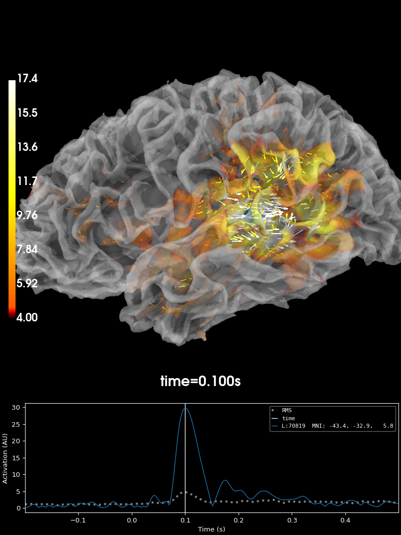
It can also be instructive to visualize the actual dipole/activation locations in 3D space in a glass brain, as opposed to activations imposed on an inflated surface (as typically done in mne.SourceEstimate.plot()), as it allows you to get a better sense of the underlying source geometry.

# Author: Marijn van Vliet <w.m.vanvliet@gmail.com>
#
# License: BSD-3-Clause
# Copyright the MNE-Python contributors.

import numpy as np

import mne
from mne.datasets import sample
from mne.minimum_norm import apply_inverse, read_inverse_operator

print(__doc__)

data_path = sample.data_path()
subjects_dir = data_path / "subjects"
smoothing_steps = 7

# Read evoked data
meg_path = data_path / "MEG" / "sample"
fname_evoked = meg_path / "sample_audvis-ave.fif"
evoked = mne.read_evokeds(fname_evoked, condition=0, baseline=(None, 0))

# Read inverse solution
fname_inv = meg_path / "sample_audvis-meg-oct-6-meg-inv.fif"
inv = read_inverse_operator(fname_inv)

# Apply inverse solution, set pick_ori='vector' to obtain a
# :class:`mne.VectorSourceEstimate` object
snr = 3.0
lambda2 = 1.0 / snr**2
stc = apply_inverse(evoked, inv, lambda2, "dSPM", pick_ori="vector")

# Use peak getter to move visualization to the time point of the peak magnitude
_, peak_time = stc.magnitude().get_peak(hemi="lh")

Reading /home/circleci/mne_data/MNE-sample-data/MEG/sample/sample_audvis-ave.fif ...
    Read a total of 4 projection items:
        PCA-v1 (1 x 102) active
        PCA-v2 (1 x 102) active
        PCA-v3 (1 x 102) active
        Average EEG reference (1 x 60) active
    Found the data of interest:
        t =    -199.80 ...     499.49 ms (Left Auditory)
        0 CTF compensation matrices available
        nave = 55 - aspect type = 100
Projections have already been applied. Setting proj attribute to True.
Applying baseline correction (mode: mean)
Reading inverse operator decomposition from /home/circleci/mne_data/MNE-sample-data/MEG/sample/sample_audvis-meg-oct-6-meg-inv.fif...
    Reading inverse operator info...
    [done]
    Reading inverse operator decomposition...
    [done]
    305 x 305 full covariance (kind = 1) found.
    Read a total of 4 projection items:
        PCA-v1 (1 x 102) active
        PCA-v2 (1 x 102) active
        PCA-v3 (1 x 102) active
        Average EEG reference (1 x 60) active
    Noise covariance matrix read.
    22494 x 22494 diagonal covariance (kind = 2) found.
    Source covariance matrix read.
    22494 x 22494 diagonal covariance (kind = 6) found.
    Orientation priors read.
    22494 x 22494 diagonal covariance (kind = 5) found.
    Depth priors read.
    Did not find the desired covariance matrix (kind = 3)
    Reading a source space...
    Computing patch statistics...
    Patch information added...
    Distance information added...
    [done]
    Reading a source space...
    Computing patch statistics...
    Patch information added...
    Distance information added...
    [done]
    2 source spaces read
    Read a total of 4 projection items:
        PCA-v1 (1 x 102) active
        PCA-v2 (1 x 102) active
        PCA-v3 (1 x 102) active
        Average EEG reference (1 x 60) active
    Source spaces transformed to the inverse solution coordinate frame
Preparing the inverse operator for use...
    Scaled noise and source covariance from nave = 1 to nave = 55
    Created the regularized inverter
    Created an SSP operator (subspace dimension = 3)
    Created the whitener using a noise covariance matrix with rank 302 (3 small eigenvalues omitted)
    Computing noise-normalization factors (dSPM)...
[done]
Applying inverse operator to "Left Auditory"...
    Picked 305 channels from the data
    Computing inverse...
    Eigenleads need to be weighted ...
    Computing residual...
    Explained  59.4% variance
    dSPM...
[done]

Plot the source estimate:

brain = stc.plot(
    initial_time=peak_time,
    hemi="lh",
    subjects_dir=subjects_dir,
    smoothing_steps=smoothing_steps,
)

# You can save a brain movie with:
# brain.save_movie(time_dilation=20, tmin=0.05, tmax=0.16, framerate=10,
#                  interpolation='linear', time_viewer=True)

Using control points [ 3.95048065  4.56941314 17.72451438]

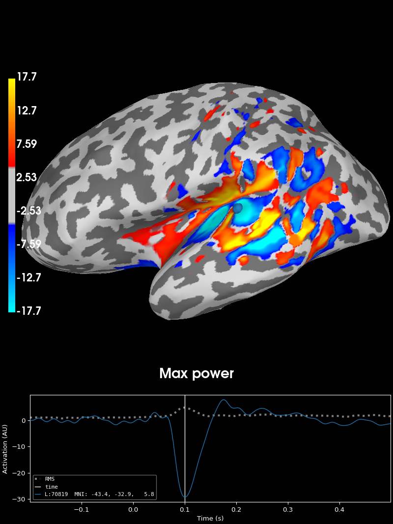
Plot the activation in the direction of maximal power for this data:

stc_max, directions = stc.project("pca", src=inv["src"])
# These directions must by design be close to the normals because this
# inverse was computed with loose=0.2
print(
    "Absolute cosine similarity between source normals and directions: "
    f'{np.abs(np.sum(directions * inv["source_nn"][2::3], axis=-1)).mean()}'
)
brain_max = stc_max.plot(
    initial_time=peak_time,
    hemi="lh",
    subjects_dir=subjects_dir,
    time_label="Max power",
    smoothing_steps=smoothing_steps,
)

Absolute cosine similarity between source normals and directions: 0.975978731472672
Using control points [ 3.90575168  4.52414196 17.71336747]

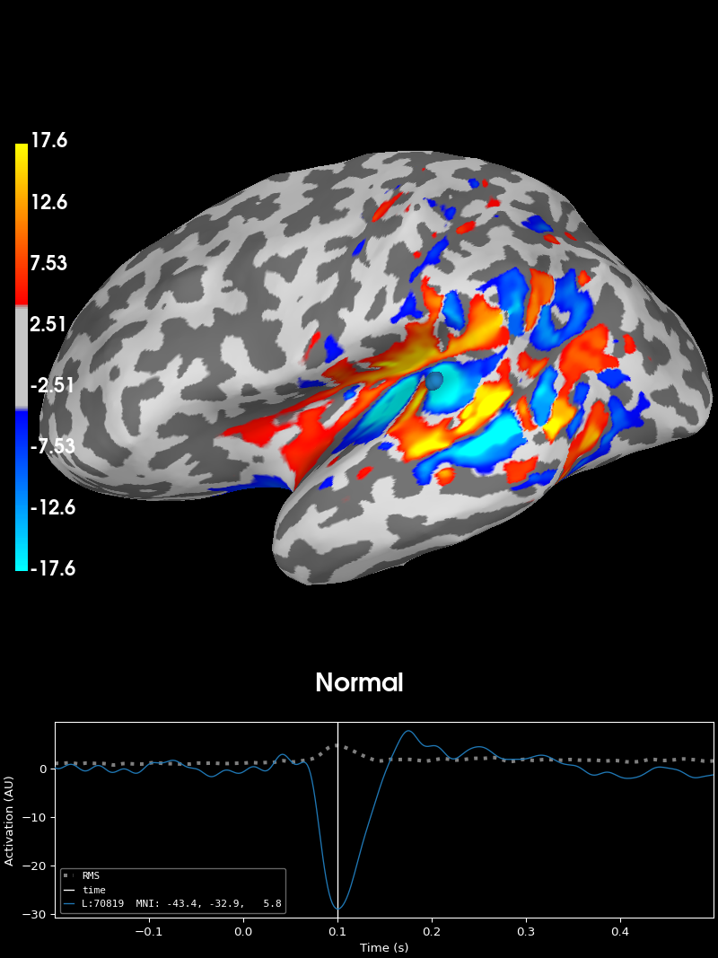
The normal is very similar:

brain_normal = stc.project("normal", inv["src"])[0].plot(
    initial_time=peak_time,
    hemi="lh",
    subjects_dir=subjects_dir,
    time_label="Normal",
    smoothing_steps=smoothing_steps,
)

Using control points [ 3.83607509  4.44726242 17.57923594]

You can also do this with a fixed-orientation inverse. It looks a lot like the result above because the loose=0.2 orientation constraint keeps sources close to fixed orientation:

fname_inv_fixed = meg_path / "sample_audvis-meg-oct-6-meg-fixed-inv.fif"
inv_fixed = read_inverse_operator(fname_inv_fixed)
stc_fixed = apply_inverse(evoked, inv_fixed, lambda2, "dSPM", pick_ori="vector")
brain_fixed = stc_fixed.plot(
    initial_time=peak_time,
    hemi="lh",
    subjects_dir=subjects_dir,
    smoothing_steps=smoothing_steps,
)

Reading inverse operator decomposition from /home/circleci/mne_data/MNE-sample-data/MEG/sample/sample_audvis-meg-oct-6-meg-fixed-inv.fif...
    Reading inverse operator info...
    [done]
    Reading inverse operator decomposition...
    [done]
    305 x 305 full covariance (kind = 1) found.
    Read a total of 4 projection items:
        PCA-v1 (1 x 102) active
        PCA-v2 (1 x 102) active
        PCA-v3 (1 x 102) active
        Average EEG reference (1 x 60) active
    Noise covariance matrix read.
    7498 x 7498 diagonal covariance (kind = 2) found.
    Source covariance matrix read.
    Did not find the desired covariance matrix (kind = 6)
    7498 x 7498 diagonal covariance (kind = 5) found.
    Depth priors read.
    Did not find the desired covariance matrix (kind = 3)
    Reading a source space...
    Computing patch statistics...
    Patch information added...
    Distance information added...
    [done]
    Reading a source space...
    Computing patch statistics...
    Patch information added...
    Distance information added...
    [done]
    2 source spaces read
    Read a total of 4 projection items:
        PCA-v1 (1 x 102) active
        PCA-v2 (1 x 102) active
        PCA-v3 (1 x 102) active
        Average EEG reference (1 x 60) active
    Source spaces transformed to the inverse solution coordinate frame
Preparing the inverse operator for use...
    Scaled noise and source covariance from nave = 1 to nave = 55
    Created the regularized inverter
    Created an SSP operator (subspace dimension = 3)
    Created the whitener using a noise covariance matrix with rank 302 (3 small eigenvalues omitted)
    Computing noise-normalization factors (dSPM)...
[done]
Applying inverse operator to "Left Auditory"...
    Picked 305 channels from the data
    Computing inverse...
    Eigenleads need to be weighted ...
    Computing residual...
    Explained  59.3% variance
    dSPM...
[done]
Using control points [ 4.00351751  4.62842071 17.43519503]