The role of dipole orientations in distributed source localization

When performing source localization in a distributed manner (i.e., using MNE/dSPM/sLORETA/eLORETA), the source space is defined as a grid of dipoles that spans a large portion of the cortex. These dipoles have both a position and an orientation. In this tutorial, we will look at the various options available to restrict the orientation of the dipoles and the impact on the resulting source estimate.

Warning

A common “gotcha!” is that by default, dipole orientation information is discarded in the source estimate. Only the magnitude of the activity is retained. This means that by default, the source-level values are always positive. This has some implications that may not be immediately obvious:

• Averaging across source estimated epochs does not produce a source estimated evoked response. Since values are always positive, noise does not “cancel out”. This means the default settings are probably not suitable for things like performing linear regression or computing correlations across epochs in source space.

• Oscillatory signals are distorted, as for example a sine wave will become a series of bumps. Hence, frequency analysis in source space is not meaningful when using the default settings.

See Orientation constraints for related information.

# Authors: The MNE-Python contributors.
# License: BSD-3-Clause
# Copyright the MNE-Python contributors.

Load data

Load everything we need to perform source localization on the sample dataset.

import numpy as np

import mne
from mne.datasets import sample
from mne.minimum_norm import apply_inverse, make_inverse_operator

data_path = sample.data_path()
meg_path = data_path / "MEG" / "sample"
evokeds = mne.read_evokeds(meg_path / "sample_audvis-ave.fif")
left_auditory = evokeds[0].apply_baseline()
fwd = mne.read_forward_solution(meg_path / "sample_audvis-meg-eeg-oct-6-fwd.fif")
mne.convert_forward_solution(fwd, surf_ori=True, copy=False)
noise_cov = mne.read_cov(meg_path / "sample_audvis-cov.fif")
subject = "sample"
subjects_dir = data_path / "subjects"
trans_fname = meg_path / "sample_audvis_raw-trans.fif"

Reading /home/circleci/mne_data/MNE-sample-data/MEG/sample/sample_audvis-ave.fif ...
    Read a total of 4 projection items:
        PCA-v1 (1 x 102) active
        PCA-v2 (1 x 102) active
        PCA-v3 (1 x 102) active
        Average EEG reference (1 x 60) active
    Found the data of interest:
        t =    -199.80 ...     499.49 ms (Left Auditory)
        0 CTF compensation matrices available
        nave = 55 - aspect type = 100
Projections have already been applied. Setting proj attribute to True.
No baseline correction applied
    Read a total of 4 projection items:
        PCA-v1 (1 x 102) active
        PCA-v2 (1 x 102) active
        PCA-v3 (1 x 102) active
        Average EEG reference (1 x 60) active
    Found the data of interest:
        t =    -199.80 ...     499.49 ms (Right Auditory)
        0 CTF compensation matrices available
        nave = 61 - aspect type = 100
Projections have already been applied. Setting proj attribute to True.
No baseline correction applied
    Read a total of 4 projection items:
        PCA-v1 (1 x 102) active
        PCA-v2 (1 x 102) active
        PCA-v3 (1 x 102) active
        Average EEG reference (1 x 60) active
    Found the data of interest:
        t =    -199.80 ...     499.49 ms (Left visual)
        0 CTF compensation matrices available
        nave = 67 - aspect type = 100
Projections have already been applied. Setting proj attribute to True.
No baseline correction applied
    Read a total of 4 projection items:
        PCA-v1 (1 x 102) active
        PCA-v2 (1 x 102) active
        PCA-v3 (1 x 102) active
        Average EEG reference (1 x 60) active
    Found the data of interest:
        t =    -199.80 ...     499.49 ms (Right visual)
        0 CTF compensation matrices available
        nave = 58 - aspect type = 100
Projections have already been applied. Setting proj attribute to True.
No baseline correction applied
Applying baseline correction (mode: mean)
Reading forward solution from /home/circleci/mne_data/MNE-sample-data/MEG/sample/sample_audvis-meg-eeg-oct-6-fwd.fif...
    Reading a source space...
    Computing patch statistics...
    Patch information added...
    Distance information added...
    [done]
    Reading a source space...
    Computing patch statistics...
    Patch information added...
    Distance information added...
    [done]
    2 source spaces read
    Desired named matrix (kind = 3523 (FIFF_MNE_FORWARD_SOLUTION_GRAD)) not available
    Read MEG forward solution (7498 sources, 306 channels, free orientations)
    Desired named matrix (kind = 3523 (FIFF_MNE_FORWARD_SOLUTION_GRAD)) not available
    Read EEG forward solution (7498 sources, 60 channels, free orientations)
    Forward solutions combined: MEG, EEG
    Source spaces transformed to the forward solution coordinate frame
    Average patch normals will be employed in the rotation to the local surface coordinates....
    Converting to surface-based source orientations...
    [done]
    366 x 366 full covariance (kind = 1) found.
    Read a total of 4 projection items:
        PCA-v1 (1 x 102) active
        PCA-v2 (1 x 102) active
        PCA-v3 (1 x 102) active
        Average EEG reference (1 x 60) active

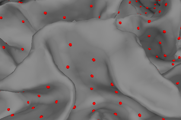
The source space

Let’s start by examining the source space as constructed by the mne.setup_source_space() function. Dipoles are placed along fixed intervals on the cortex, determined by the spacing parameter. The source space does not define the orientation for these dipoles.

lh = fwd["src"][0]  # Visualize the left hemisphere
verts = lh["rr"]  # The vertices of the source space
tris = lh["tris"]  # Groups of three vertices that form triangles
dip_pos = lh["rr"][lh["vertno"]]  # The position of the dipoles
dip_ori = lh["nn"][lh["vertno"]]
dip_len = len(dip_pos)
dip_times = [0]
white = (1.0, 1.0, 1.0)  # RGB values for a white color

actual_amp = np.ones(dip_len)  # fake amp, needed to create Dipole instance
actual_gof = np.ones(dip_len)  # fake GOF, needed to create Dipole instance
dipoles = mne.Dipole(dip_times, dip_pos, actual_amp, dip_ori, actual_gof)
trans = mne.read_trans(trans_fname)

fig = mne.viz.create_3d_figure(size=(600, 400), bgcolor=white)
coord_frame = "mri"

# Plot the cortex
mne.viz.plot_alignment(
    subject=subject,
    subjects_dir=subjects_dir,
    trans=trans,
    surfaces="white",
    coord_frame=coord_frame,
    fig=fig,
)

# Mark the position of the dipoles with small red dots
mne.viz.plot_dipole_locations(
    dipoles=dipoles,
    trans=trans,
    mode="sphere",
    subject=subject,
    subjects_dir=subjects_dir,
    coord_frame=coord_frame,
    scale=7e-4,
    fig=fig,
)

mne.viz.set_3d_view(figure=fig, azimuth=180, distance=0.1, focalpoint="auto")

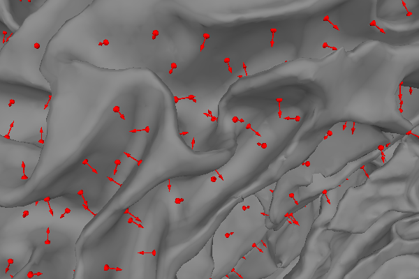
Fixed dipole orientations

While the source space defines the position of the dipoles, the inverse operator defines the possible orientations of them. One of the options is to assign a fixed orientation. Since the neural currents from which MEG and EEG signals originate flows mostly perpendicular to the cortex [1], restricting the orientation of the dipoles accordingly places a useful restriction on the source estimate.

By specifying fixed=True when calling mne.minimum_norm.make_inverse_operator(), the dipole orientations are fixed to be orthogonal to the surface of the cortex, pointing outwards. Let’s visualize this:

fig = mne.viz.create_3d_figure(size=(600, 400))

# Plot the cortex
mne.viz.plot_alignment(
    subject=subject,
    subjects_dir=subjects_dir,
    trans=trans,
    surfaces="white",
    coord_frame="head",
    fig=fig,
)

# Show the dipoles as arrows pointing along the surface normal
mne.viz.plot_dipole_locations(
    dipoles=dipoles,
    trans=trans,
    mode="arrow",
    subject=subject,
    subjects_dir=subjects_dir,
    coord_frame="head",
    scale=7e-4,
    fig=fig,
)

mne.viz.set_3d_view(figure=fig, azimuth=180, distance=0.1, focalpoint="auto")

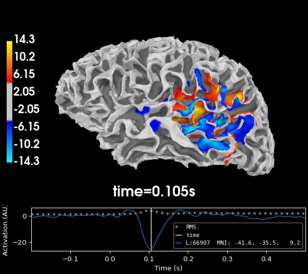
Restricting the dipole orientations in this manner leads to the following source estimate for the sample data:

# Compute the source estimate for the left auditory condition in the sample
# dataset.
inv = make_inverse_operator(left_auditory.info, fwd, noise_cov, fixed=True)
stc = apply_inverse(left_auditory, inv, pick_ori=None)

# Visualize it at the moment of peak activity.
_, time_max = stc.get_peak(hemi="lh")
brain_fixed = stc.plot(
    surface="white",
    subjects_dir=subjects_dir,
    initial_time=time_max,
    time_unit="s",
    size=(600, 400),
)
mne.viz.set_3d_view(figure=brain_fixed, focalpoint=(0.0, 0.0, 50))

Computing inverse operator with 364 channels.
    364 out of 366 channels remain after picking
Selected 364 channels
Creating the depth weighting matrix...
    203 planar channels
    limit = 7262/7498 = 10.020865
    scale = 2.58122e-08 exp = 0.8
    Picked elements from a free-orientation depth-weighting prior into the fixed-orientation one
    Average patch normals will be employed in the rotation to the local surface coordinates....
    Converting to surface-based source orientations...
    [done]
Whitening the forward solution.
    Created an SSP operator (subspace dimension = 4)
Computing rank from covariance with rank=None
    Using tolerance 3.3e-13 (2.2e-16 eps * 305 dim * 4.8  max singular value)
    Estimated rank (mag + grad): 302
    MEG: rank 302 computed from 305 data channels with 3 projectors
    Using tolerance 4.7e-14 (2.2e-16 eps * 59 dim * 3.6  max singular value)
    Estimated rank (eeg): 58
    EEG: rank 58 computed from 59 data channels with 1 projector
    Setting small MEG eigenvalues to zero (without PCA)
    Setting small EEG eigenvalues to zero (without PCA)
Creating the source covariance matrix
Adjusting source covariance matrix.
Computing SVD of whitened and weighted lead field matrix.
    largest singular value = 5.70263
    scaling factor to adjust the trace = 1.18949e+19 (nchan = 364 nzero = 4)
Preparing the inverse operator for use...
    Scaled noise and source covariance from nave = 1 to nave = 55
    Created the regularized inverter
    Created an SSP operator (subspace dimension = 4)
    Created the whitener using a noise covariance matrix with rank 360 (4 small eigenvalues omitted)
    Computing noise-normalization factors (dSPM)...
[done]
Applying inverse operator to "Left Auditory"...
    Picked 364 channels from the data
    Computing inverse...
    Eigenleads need to be weighted ...
    Computing residual...
    Explained  64.5% variance
    dSPM...
[done]
Using control points [ 4.06165525  4.70033915 14.34794621]

The direction of the estimated current is now restricted to two directions: inward and outward. In the plot, blue areas indicate current flowing inwards and red areas indicate current flowing outwards. Given the curvature of the cortex, groups of dipoles tend to point in the same direction: the direction of the electromagnetic field picked up by the sensors.

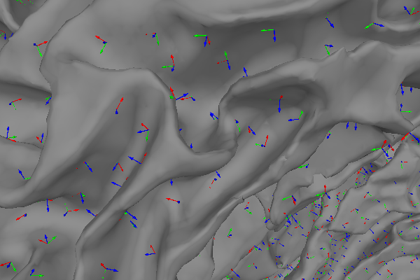
Loose dipole orientations

Forcing the source dipoles to be strictly orthogonal to the cortex makes the source estimate sensitive to the spacing of the dipoles along the cortex, since the curvature of the cortex changes within each ~10 square mm patch. Furthermore, misalignment of the MEG/EEG and MRI coordinate frames is more critical when the source dipole orientations are strictly constrained [2]. To lift the restriction on the orientation of the dipoles, the inverse operator has the ability to place not one, but three dipoles at each location defined by the source space. These three dipoles are placed orthogonally to form a Cartesian coordinate system. Let’s visualize this:

fig = mne.viz.create_3d_figure(size=(600, 400))

# Plot the cortex
mne.viz.plot_alignment(
    subject=subject,
    subjects_dir=subjects_dir,
    trans=trans,
    surfaces="white",
    coord_frame="head",
    fig=fig,
)

# Show the three dipoles defined at each location in the source space
mne.viz.plot_alignment(
    subject=subject,
    subjects_dir=subjects_dir,
    trans=trans,
    fwd=fwd,
    surfaces="white",
    coord_frame="head",
    fig=fig,
)

mne.viz.set_3d_view(figure=fig, azimuth=180, distance=0.1, focalpoint="auto")

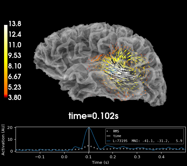
When computing the source estimate, the activity at each of the three dipoles is collapsed into the XYZ components of a single vector, which leads to the following source estimate for the sample data:

# Make an inverse operator with loose dipole orientations
inv = make_inverse_operator(left_auditory.info, fwd, noise_cov, fixed=False, loose=1.0)

# Compute the source estimate, indicate that we want a vector solution
stc = apply_inverse(left_auditory, inv, pick_ori="vector")

# Visualize it at the moment of peak activity.
_, time_max = stc.magnitude().get_peak(hemi="lh")
brain_mag = stc.plot(
    subjects_dir=subjects_dir,
    initial_time=time_max,
    time_unit="s",
    size=(600, 400),
    overlay_alpha=0,
)
mne.viz.set_3d_view(figure=brain_mag, focalpoint=(0.0, 0.0, 50))

Computing inverse operator with 364 channels.
    364 out of 366 channels remain after picking
Selected 364 channels
Creating the depth weighting matrix...
    203 planar channels
    limit = 7262/7498 = 10.020865
    scale = 2.58122e-08 exp = 0.8
Whitening the forward solution.
    Created an SSP operator (subspace dimension = 4)
Computing rank from covariance with rank=None
    Using tolerance 3.3e-13 (2.2e-16 eps * 305 dim * 4.8  max singular value)
    Estimated rank (mag + grad): 302
    MEG: rank 302 computed from 305 data channels with 3 projectors
    Using tolerance 4.7e-14 (2.2e-16 eps * 59 dim * 3.6  max singular value)
    Estimated rank (eeg): 58
    EEG: rank 58 computed from 59 data channels with 1 projector
    Setting small MEG eigenvalues to zero (without PCA)
    Setting small EEG eigenvalues to zero (without PCA)
Creating the source covariance matrix
Adjusting source covariance matrix.
Computing SVD of whitened and weighted lead field matrix.
    largest singular value = 5.2188
    scaling factor to adjust the trace = 3.44205e+19 (nchan = 364 nzero = 4)
Preparing the inverse operator for use...
    Scaled noise and source covariance from nave = 1 to nave = 55
    Created the regularized inverter
    Created an SSP operator (subspace dimension = 4)
    Created the whitener using a noise covariance matrix with rank 360 (4 small eigenvalues omitted)
    Computing noise-normalization factors (dSPM)...
[done]
Applying inverse operator to "Left Auditory"...
    Picked 364 channels from the data
    Computing inverse...
    Eigenleads need to be weighted ...
    Computing residual...
    Explained  64.8% variance
    dSPM...
[done]
Using control points [ 3.79973942  4.38378769 13.8347911 ]

Limiting orientations, but not fixing them

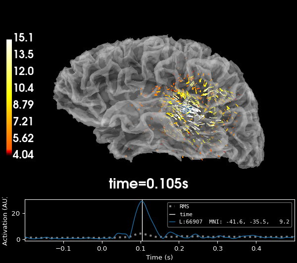
Often, the best results will be obtained by allowing the dipoles to have somewhat free orientation, but not stray too far from a orientation that is perpendicular to the cortex. The loose parameter of the mne.minimum_norm.make_inverse_operator() allows you to specify a value between 0 (fixed) and 1 (unrestricted or “free”) to indicate the amount the orientation is allowed to deviate from the surface normal.

# Set loose to 0.2, the default value
inv = make_inverse_operator(left_auditory.info, fwd, noise_cov, fixed=False, loose=0.2)
stc = apply_inverse(left_auditory, inv, pick_ori="vector")

# Visualize it at the moment of peak activity.
_, time_max = stc.magnitude().get_peak(hemi="lh")
brain_loose = stc.plot(
    subjects_dir=subjects_dir,
    initial_time=time_max,
    time_unit="s",
    size=(600, 400),
    overlay_alpha=0,
)
mne.viz.set_3d_view(figure=brain_loose, focalpoint=(0.0, 0.0, 50))

Computing inverse operator with 364 channels.
    364 out of 366 channels remain after picking
Selected 364 channels
Creating the depth weighting matrix...
    203 planar channels
    limit = 7262/7498 = 10.020865
    scale = 2.58122e-08 exp = 0.8
Applying loose dipole orientations to surface source spaces: 0.2
Whitening the forward solution.
    Created an SSP operator (subspace dimension = 4)
Computing rank from covariance with rank=None
    Using tolerance 3.3e-13 (2.2e-16 eps * 305 dim * 4.8  max singular value)
    Estimated rank (mag + grad): 302
    MEG: rank 302 computed from 305 data channels with 3 projectors
    Using tolerance 4.7e-14 (2.2e-16 eps * 59 dim * 3.6  max singular value)
    Estimated rank (eeg): 58
    EEG: rank 58 computed from 59 data channels with 1 projector
    Setting small MEG eigenvalues to zero (without PCA)
    Setting small EEG eigenvalues to zero (without PCA)
Creating the source covariance matrix
Adjusting source covariance matrix.
Computing SVD of whitened and weighted lead field matrix.
    largest singular value = 5.49264
    scaling factor to adjust the trace = 1.64e+19 (nchan = 364 nzero = 4)
Preparing the inverse operator for use...
    Scaled noise and source covariance from nave = 1 to nave = 55
    Created the regularized inverter
    Created an SSP operator (subspace dimension = 4)
    Created the whitener using a noise covariance matrix with rank 360 (4 small eigenvalues omitted)
    Computing noise-normalization factors (dSPM)...
[done]
Applying inverse operator to "Left Auditory"...
    Picked 364 channels from the data
    Computing inverse...
    Eigenleads need to be weighted ...
    Computing residual...
    Explained  64.8% variance
    dSPM...
[done]
Using control points [ 4.03844879  4.68532258 15.12541436]

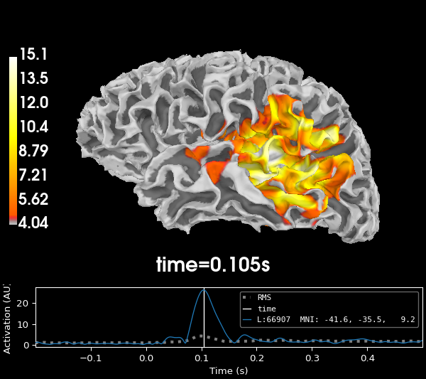
Discarding dipole orientation information

Often, further analysis of the data does not need information about the orientation of the dipoles, but rather their magnitudes. The pick_ori parameter of the mne.minimum_norm.apply_inverse() function allows you to specify whether to return the full vector solution ('vector') or rather the magnitude of the vectors (None, the default) or only the activity in the direction perpendicular to the cortex ('normal').

# Only retain vector magnitudes
stc = apply_inverse(left_auditory, inv, pick_ori=None)

# Visualize it at the moment of peak activity
_, time_max = stc.get_peak(hemi="lh")
brain = stc.plot(
    surface="white",
    subjects_dir=subjects_dir,
    initial_time=time_max,
    time_unit="s",
    size=(600, 400),
)
mne.viz.set_3d_view(figure=brain, focalpoint=(0.0, 0.0, 50))

Preparing the inverse operator for use...
    Scaled noise and source covariance from nave = 1 to nave = 55
    Created the regularized inverter
    Created an SSP operator (subspace dimension = 4)
    Created the whitener using a noise covariance matrix with rank 360 (4 small eigenvalues omitted)
    Computing noise-normalization factors (dSPM)...
[done]
Applying inverse operator to "Left Auditory"...
    Picked 364 channels from the data
    Computing inverse...
    Eigenleads need to be weighted ...
    Computing residual...
    Explained  64.8% variance
    Combining the current components...
    dSPM...
[done]
Using control points [ 4.03844879  4.68532258 15.12541436]

References

[1]

Matti S. Hämäläinen, Riitta Hari, Risto J. Ilmoniemi, Jukka Knuutila, and Olli V. Lounasmaa. Magnetoencephalography—theory, instrumentation, and applications to noninvasive studies of the working human brain. Reviews of Modern Physics, 65(2):413–497, 1993. doi:10.1103/RevModPhys.65.413.

[2]

Fa-Hsuan Lin, John W. Belliveau, Anders M. Dale, and Matti S. Hämäläinen. Distributed current estimates using cortical orientation constraints. Human Brain Mapping, 27(1):1–13, 2006. doi:10.1002/hbm.20155.