Note
Go to the end to download the full example code.
Compare simulated and estimated source activity#
This example illustrates how to compare the simulated and estimated source time courses (STC) by computing different metrics. Simulated source is a cortical region or dipole. It is meant to be a brief introduction and only highlights the simplest use case.
# Author: Kostiantyn Maksymenko <kostiantyn.maksymenko@gmail.com>
#
# License: BSD-3-Clause
# Copyright the MNE-Python contributors.

from functools import partial

import matplotlib.pyplot as plt
import numpy as np

import mne
from mne.datasets import sample
from mne.minimum_norm import apply_inverse, make_inverse_operator
from mne.simulation.metrics import (
    cosine_score,
    f1_score,
    peak_position_error,
    precision_score,
    recall_score,
    region_localization_error,
    spatial_deviation_error,
)

random_state = 42  # set random state to make this example deterministic

# Import sample data
data_path = sample.data_path()
subjects_dir = data_path / "subjects"
subject = "sample"
evoked_fname = data_path / "MEG" / subject / "sample_audvis-ave.fif"
info = mne.io.read_info(evoked_fname)
tstep = 1.0 / info["sfreq"]

# Import forward operator and source space
fwd_fname = data_path / "MEG" / subject / "sample_audvis-meg-eeg-oct-6-fwd.fif"
fwd = mne.read_forward_solution(fwd_fname)
src = fwd["src"]

# To select source, we use the caudal middle frontal to grow
# a region of interest.
selected_label = mne.read_labels_from_annot(
    subject, regexp="caudalmiddlefrontal-lh", subjects_dir=subjects_dir
)[0]
    Read a total of 4 projection items:
        PCA-v1 (1 x 10²) active
        PCA-v2 (1 x 10²) active
        PCA-v3 (1 x 10²) active
        Average EEG reference (1 x 60) active
Reading forward solution from /home/circleci/mne_data/MNE-sample-data/MEG/sample/sample_audvis-meg-eeg-oct-6-fwd.fif...
    Reading a source space...
    Computing patch statistics...
    Patch information added...
    Distance information added...
    [done]
    Reading a source space...
    Computing patch statistics...
    Patch information added...
    Distance information added...
    [done]
    2 source spaces read
    Desired named matrix (kind = 3523 (FIFF_MNE_FORWARD_SOLUTION_GRAD)) not available
    Read MEG forward solution (7498 sources, 306 channels, free orientations)
    Desired named matrix (kind = 3523 (FIFF_MNE_FORWARD_SOLUTION_GRAD)) not available
    Read EEG forward solution (7498 sources, 60 channels, free orientations)
    Forward solutions combined: MEG, EEG
    Source spaces transformed to the forward solution coordinate frame
Reading labels from parcellation...
   read 1 labels from /home/circleci/mne_data/MNE-sample-data/subjects/sample/label/lh.aparc.annot
   read 0 labels from /home/circleci/mne_data/MNE-sample-data/subjects/sample/label/rh.aparc.annot
In this example we simulate two types of cortical sources: a region and a dipole sources. We will test corresponding performance metrics.
Define main parameters of sources#
First we define both region and dipole sources in terms of Where?, What? and When?.
# WHERE?

# Region
location = "center"  # Use the center of the label as a seed.
extent = 20.0  # Extent in mm of the region.
label_region = mne.label.select_sources(
    subject,
    selected_label,
    location=location,
    extent=extent,
    subjects_dir=subjects_dir,
    random_state=random_state,
)

# Dipole
location = 1915  # Use the index of the vertex as a seed
extent = 0.0  # One dipole source
label_dipole = mne.label.select_sources(
    subject,
    selected_label,
    location=location,
    extent=extent,
    subjects_dir=subjects_dir,
    random_state=random_state,
)

# WHAT?
# Define the time course of the activity
source_time_series = np.sin(2.0 * np.pi * 18.0 * np.arange(100) * tstep) * 10e-9

# WHEN?
# Define when the activity occurs using events.
n_events = 50
events = np.zeros((n_events, 3), int)
events[:, 0] = 200 * np.arange(n_events)  # Events sample.
events[:, 2] = 1  # All events have the sample id.
Create simulated source activity#
Here, SourceSimulator is used.
# Region
source_simulator_region = mne.simulation.SourceSimulator(src, tstep=tstep)
source_simulator_region.add_data(label_region, source_time_series, events)

# Dipole
source_simulator_dipole = mne.simulation.SourceSimulator(src, tstep=tstep)
source_simulator_dipole.add_data(label_dipole, source_time_series, events)
Simulate raw data#
Project the source time series to sensor space with multivariate Gaussian noise obtained from the noise covariance from the sample data.
# Region
raw_region = mne.simulation.simulate_raw(info, source_simulator_region, forward=fwd)
raw_region = raw_region.pick(picks=["eeg", "stim"], exclude="bads")
cov = mne.make_ad_hoc_cov(raw_region.info)
mne.simulation.add_noise(
    raw_region, cov, iir_filter=[0.2, -0.2, 0.04], random_state=random_state
)

# Dipole
raw_dipole = mne.simulation.simulate_raw(info, source_simulator_dipole, forward=fwd)
raw_dipole = raw_dipole.pick(picks=["eeg", "stim"], exclude="bads")
cov = mne.make_ad_hoc_cov(raw_dipole.info)
mne.simulation.add_noise(
    raw_dipole, cov, iir_filter=[0.2, -0.2, 0.04], random_state=random_state
)
Setting up raw simulation: 1 position, "cos2" interpolation
Event information stored on channel:              STI 014
    Interval 0.000–1.665 s
Setting up forward solutions
Computing gain matrix for transform #1/1
    Interval 0.000–1.665 s
    Interval 0.000–1.665 s
    Interval 0.000–1.665 s
    Interval 0.000–1.665 s
    Interval 0.000–1.665 s
    Interval 0.000–1.665 s
    Interval 0.000–1.665 s
    Interval 0.000–1.665 s
    Interval 0.000–1.498 s
    10 STC iterations provided
[done]
Adding noise to 59/68 channels (59 channels in cov)
Compute evoked from raw data#
Averaging epochs corresponding to events.
# Region
events = mne.find_events(raw_region, initial_event=True)
tmax = (len(source_time_series) - 1) * tstep
epochs = mne.Epochs(raw_region, events, 1, tmin=0, tmax=tmax, baseline=None)
evoked_region = epochs.average()

# Dipole
events = mne.find_events(raw_dipole, initial_event=True)
tmax = (len(source_time_series) - 1) * tstep
epochs = mne.Epochs(raw_dipole, events, 1, tmin=0, tmax=tmax, baseline=None)
evoked_dipole = epochs.average()
Finding events on: STI 014
50 events found on stim channel STI 014
Event IDs: [1]
Not setting metadata
50 matching events found
No baseline correction applied
Created an SSP operator (subspace dimension = 1)
1 projection items activated
Finding events on: STI 014
50 events found on stim channel STI 014
Event IDs: [1]
Not setting metadata
50 matching events found
No baseline correction applied
Created an SSP operator (subspace dimension = 1)
1 projection items activated
Create true stcs corresponding to evoked#
Before we computed stcs corresponding to raw data. To be able to compare it with the reconstruction, based on the evoked, true stc should have the same number of time samples.
# Region
stc_true_region = source_simulator_region.get_stc(
    start_sample=0, stop_sample=len(source_time_series)
)

# Dipole
stc_true_dipole = source_simulator_dipole.get_stc(
    start_sample=0, stop_sample=len(source_time_series)
)
Reconstruct simulated sources#
Compute inverse solution using sLORETA.
# Region
snr = 30.0
inv_method = "sLORETA"
lambda2 = 1.0 / snr**2

inverse_operator = make_inverse_operator(
    evoked_region.info, fwd, cov, loose="auto", depth=0.8, fixed=True
)

stc_est_region = apply_inverse(
    evoked_region, inverse_operator, lambda2, inv_method, pick_ori=None
)

# Dipole
snr = 3.0
inv_method = "sLORETA"
lambda2 = 1.0 / snr**2

inverse_operator = make_inverse_operator(
    evoked_dipole.info, fwd, cov, loose="auto", depth=0.8, fixed=True
)

stc_est_dipole = apply_inverse(
    evoked_dipole, inverse_operator, lambda2, inv_method, pick_ori=None
)
Computing inverse operator with 59 channels.
    59 out of 366 channels remain after picking
Selected 59 channels
Creating the depth weighting matrix...
    59 EEG channels
    limit = 7499/7498 = 2.118742
    scale = 155292 exp = 0.8
    Picked elements from a free-orientation depth-weighting prior into the fixed-orientation one
    Average patch normals will be employed in the rotation to the local surface coordinates....
    Converting to surface-based source orientations...
    [done]
Whitening the forward solution.
    Created an SSP operator (subspace dimension = 1)
Computing rank from covariance with rank=None
    Using tolerance 5.2e-18 (2.2e-16 eps * 59 dim * 0.0004  max singular value)
    Estimated rank (eeg): 58
    EEG: rank 58 computed from 59 data channels with 1 projector
    Setting small EEG eigenvalues to zero (without PCA)
Creating the source covariance matrix
Adjusting source covariance matrix.
Computing SVD of whitened and weighted lead field matrix.
    largest singular value = 4.2931
    scaling factor to adjust the trace = 1.34986e+22 (nchan = 59 nzero = 1)
Preparing the inverse operator for use...
    Scaled noise and source covariance from nave = 1 to nave = 50
    Created the regularized inverter
    Created an SSP operator (subspace dimension = 1)
    Created the whitener using a noise covariance matrix with rank 58 (1 small eigenvalues omitted)
    Computing noise-normalization factors (sLORETA)...
[done]
Applying inverse operator to "1"...
    Picked 59 channels from the data
    Computing inverse...
    Eigenleads need to be weighted ...
    Computing residual...
    Explained 100.0% variance
    sLORETA...
[done]
Computing inverse operator with 59 channels.
    59 out of 366 channels remain after picking
Selected 59 channels
Creating the depth weighting matrix...
    59 EEG channels
    limit = 7499/7498 = 2.118742
    scale = 155292 exp = 0.8
    Picked elements from a free-orientation depth-weighting prior into the fixed-orientation one
    Average patch normals will be employed in the rotation to the local surface coordinates....
    Converting to surface-based source orientations...
    [done]
Whitening the forward solution.
    Created an SSP operator (subspace dimension = 1)
Computing rank from covariance with rank=None
    Using tolerance 5.2e-18 (2.2e-16 eps * 59 dim * 0.0004  max singular value)
    Estimated rank (eeg): 58
    EEG: rank 58 computed from 59 data channels with 1 projector
    Setting small EEG eigenvalues to zero (without PCA)
Creating the source covariance matrix
Adjusting source covariance matrix.
Computing SVD of whitened and weighted lead field matrix.
    largest singular value = 4.2931
    scaling factor to adjust the trace = 1.34986e+22 (nchan = 59 nzero = 1)
Preparing the inverse operator for use...
    Scaled noise and source covariance from nave = 1 to nave = 50
    Created the regularized inverter
    Created an SSP operator (subspace dimension = 1)
    Created the whitener using a noise covariance matrix with rank 58 (1 small eigenvalues omitted)
    Computing noise-normalization factors (sLORETA)...
[done]
Applying inverse operator to "1"...
    Picked 59 channels from the data
    Computing inverse...
    Eigenleads need to be weighted ...
    Computing residual...
    Explained  85.5% variance
    sLORETA...
[done]
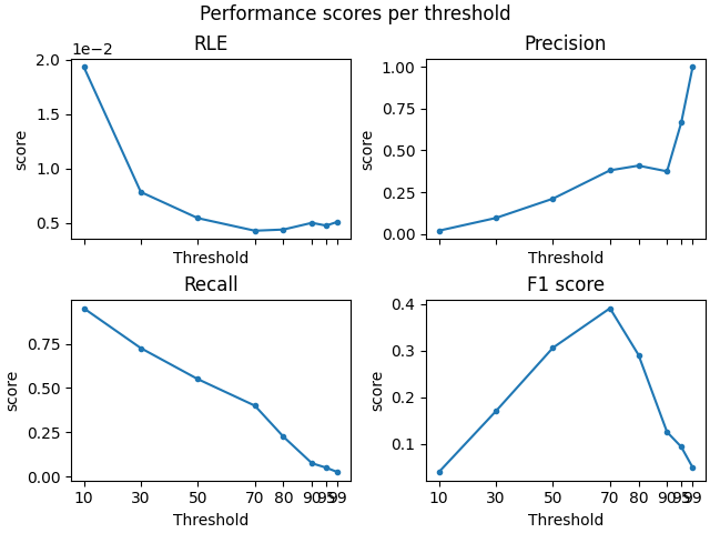
Compute performance scores for different source amplitude thresholds#
thresholds = [10, 30, 50, 70, 80, 90, 95, 99]
For region#
# create a set of scorers
scorers = {
"RLE": partial(region_localization_error, src=src),
"Precision": precision_score,
"Recall": recall_score,
"F1 score": f1_score,
}
# compute results
region_results = {}
for name, scorer in scorers.items():
region_results[name] = [
scorer(stc_true_region, stc_est_region, threshold=f"{thx}%", per_sample=False)
for thx in thresholds
]
# Plot the results
f, ((ax1, ax2), (ax3, ax4)) = plt.subplots(2, 2, sharex="col", layout="constrained")
for ax, (title, results) in zip([ax1, ax2, ax3, ax4], region_results.items()):
ax.plot(thresholds, results, ".-")
ax.set(title=title, ylabel="score", xlabel="Threshold", xticks=thresholds)
f.suptitle("Performance scores per threshold") # Add Super title
ax1.ticklabel_format(axis="y", style="sci", scilimits=(0, 1)) # tweak RLE
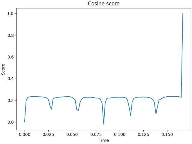
# Cosine score with respect to time
f, ax1 = plt.subplots(layout="constrained")
ax1.plot(stc_true_region.times, cosine_score(stc_true_region, stc_est_region))
ax1.set(title="Cosine score", xlabel="Time", ylabel="Score")
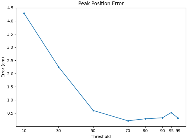
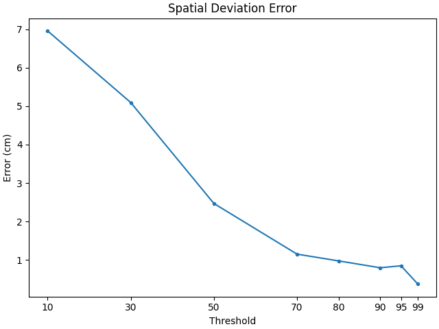
For Dipoles#
# create a set of scorers
scorers = {
    "Peak Position Error": peak_position_error,
    "Spatial Deviation Error": spatial_deviation_error,
}


# compute results
dipole_results = {}
for name, scorer in scorers.items():
    dipole_results[name] = [
        scorer(
            stc_true_dipole,
            stc_est_dipole,
            src=src,
            threshold=f"{thx}%",
            per_sample=False,
        )
        for thx in thresholds
    ]


# Plot the results
for name, results in dipole_results.items():
    f, ax1 = plt.subplots(layout="constrained")
    ax1.plot(thresholds, 100 * np.array(results), ".-")
    ax1.set(title=name, ylabel="Error (cm)", xlabel="Threshold", xticks=thresholds)
Total running time of the script: (0 minutes 8.909 seconds)