Note
Go to the end to download the full example code.
Computing source timecourses with an XFit-like multi-dipole model#
MEGIN’s XFit program offers a “guided ECD modeling” interface, where multiple dipoles can be fitted interactively. By manually selecting subsets of sensors and time ranges, dipoles can be fitted to specific signal components. Then, source timecourses can be computed using a multi-dipole model. The advantage of using a multi-dipole model over fitting each dipole in isolation, is that when multiple dipoles contribute to the same signal component, the model can make sure that activity assigned to one dipole is not also assigned to another. This example shows how to build a multi-dipole model for estimating source timecourses for evokeds or single epochs.
The XFit program is the recommended approach for guided ECD modeling, because
it offers a convenient graphical user interface for it. These dipoles can then
be imported into MNE-Python by using the mne.read_dipole() function for
building and applying the multi-dipole model. In addition, this example will
also demonstrate how to perform guided ECD modeling using only MNE-Python
functionality, which is less convenient than using XFit, but has the benefit of
being reproducible.
# Author: Marijn van Vliet <w.m.vanvliet@gmail.com>
#
# License: BSD-3-Clause
# Copyright the MNE-Python contributors.
Importing everything and setting up the data paths for the MNE-Sample dataset.
import matplotlib.pyplot as plt
import numpy as np

import mne
from mne.channels import read_vectorview_selection
from mne.datasets import sample
from mne.minimum_norm import apply_inverse, apply_inverse_epochs, make_inverse_operator

data_path = sample.data_path()
meg_path = data_path / "MEG" / "sample"
raw_fname = meg_path / "sample_audvis_raw.fif"
cov_fname = meg_path / "sample_audvis-shrunk-cov.fif"
bem_dir = data_path / "subjects" / "sample" / "bem"
bem_fname = bem_dir / "sample-5120-5120-5120-bem-sol.fif"
trans_fname = meg_path / "sample_audvis_raw-trans.fif"
Read the MEG data from the audvis experiment. Make epochs and evokeds for the left and right auditory conditions.
raw = mne.io.read_raw_fif(raw_fname)
raw = raw.pick(picks=["meg", "eog", "stim"])
info = raw.info

# Create epochs for auditory events
events = mne.find_events(raw)
event_id = dict(right=1, left=2)
epochs = mne.Epochs(
    raw,
    events,
    event_id,
    tmin=-0.1,
    tmax=0.3,
    baseline=(None, 0),
    reject=dict(mag=4e-12, grad=4000e-13, eog=150e-6),
)

# Create evokeds for left and right auditory stimulation
evoked_left = epochs["left"].average()
evoked_right = epochs["right"].average()
Opening raw data file /home/circleci/mne_data/MNE-sample-data/MEG/sample/sample_audvis_raw.fif...
    Read a total of 3 projection items:
        PCA-v1 (1 x 10²)  idle
        PCA-v2 (1 x 10²)  idle
        PCA-v3 (1 x 10²)  idle
    Range : 25800 ... 192599 =     42.956 ...   320.670 secs
Ready.
Finding events on: STI 014
320 events found on stim channel STI 014
Event IDs: [ 1  2  3  4  5 32]
Not setting metadata
145 matching events found
Setting baseline interval to [-0.09989760657919393, 0.0] s
Applying baseline correction (mode: mean)
Created an SSP operator (subspace dimension = 3)
3 projection items activated
    Rejecting  epoch based on EOG : ['EOG 061']
    Rejecting  epoch based on EOG : ['EOG 061']
    Rejecting  epoch based on EOG : ['EOG 061']
    Rejecting  epoch based on EOG : ['EOG 061']
    Rejecting  epoch based on EOG : ['EOG 061']
    Rejecting  epoch based on EOG : ['EOG 061']
    Rejecting  epoch based on EOG : ['EOG 061']
    Rejecting  epoch based on EOG : ['EOG 061']
    Rejecting  epoch based on EOG : ['EOG 061']
    Rejecting  epoch based on MAG : ['MEG 1711']
    Rejecting  epoch based on EOG : ['EOG 061']
    Rejecting  epoch based on EOG : ['EOG 061']
    Rejecting  epoch based on EOG : ['EOG 061']
    Rejecting  epoch based on EOG : ['EOG 061']
Guided dipole modeling, meaning fitting dipoles to a manually selected subset of sensors as a manually chosen time, can now be performed in MEGINs XFit on the evokeds we computed above. However, it is possible to do it completely in MNE-Python.
# Setup conductor model
cov = mne.read_cov(cov_fname)  # bad channels were already excluded here
bem = mne.read_bem_solution(bem_fname)

# Fit two dipoles at t=80ms. The first dipole is fitted using only the sensors
# on the left side of the helmet. The second dipole is fitted using only the
# sensors on the right side of the helmet.
picks_left = read_vectorview_selection("Left", info=info)
evoked_fit_left = evoked_left.copy().crop(0.08, 0.08)
evoked_fit_left.pick(picks_left)
cov_fit_left = cov.copy().pick_channels(picks_left, ordered=True)

picks_right = read_vectorview_selection("Right", info=info)
picks_right = list(set(picks_right) - set(info["bads"]))
evoked_fit_right = evoked_right.copy().crop(0.08, 0.08)
evoked_fit_right.pick(picks_right)
cov_fit_right = cov.copy().pick_channels(picks_right, ordered=True)

# Any SSS projections that are active on this data need to be re-normalized
# after picking channels.
evoked_fit_left.info.normalize_proj()
evoked_fit_right.info.normalize_proj()
cov_fit_left["projs"] = evoked_fit_left.info["projs"]
cov_fit_right["projs"] = evoked_fit_right.info["projs"]

# Fit the dipoles with the subset of sensors.
kwargs = dict(bem=bem, trans=trans_fname)
dip_left, _ = mne.fit_dipole(evoked_fit_left, cov_fit_left, **kwargs)
dip_right, _ = mne.fit_dipole(evoked_fit_right, cov_fit_right, **kwargs)
    365 x 365 full covariance (kind = 1) found.
    Read a total of 4 projection items:
        PCA-v1 (1 x 10²) active
        PCA-v2 (1 x 10²) active
        PCA-v3 (1 x 10²) active
        Average EEG reference (1 x 59) active
Loading surfaces...

Loading the solution matrix...

Three-layer model surfaces loaded.
Loaded linear collocation BEM solution from /home/circleci/mne_data/MNE-sample-data/subjects/sample/bem/sample-5120-5120-5120-bem-sol.fif
BEM               : <ConductorModel | BEM (3 layers) solver=mne>
MRI transform     : /home/circleci/mne_data/MNE-sample-data/MEG/sample/sample_audvis_raw-trans.fif
Head origin       :   -4.2   19.3   65.3 mm rad =   72.3 mm.
Guess grid        :   20.0 mm
Guess mindist     :    5.0 mm
Guess exclude     :   20.0 mm
Using normal MEG coil definitions.
Noise covariance  : <Covariance | kind : full, shape : (153, 153), range : [-1.4e-23, +3.7e-23], n_samples : 38720>

Coordinate transformation: MRI (surface RAS) -> head
    0.999310 0.009985 -0.035787      -3.17 mm
    0.012759 0.812405 0.582954       6.86 mm
    0.034894 -0.583008 0.811716      28.88 mm
    0.000000 0.000000 0.000000       1.00
Coordinate transformation: MEG device -> head
    0.991420 -0.039936 -0.124467      -6.13 mm
    0.060661 0.984012 0.167456       0.06 mm
    0.115790 -0.173570 0.977991      64.74 mm
    0.000000 0.000000 0.000000       1.00
0 bad channels total
Read 153 MEG channels from info
105 coil definitions read
Coordinate transformation: MEG device -> head
    0.991420 -0.039936 -0.124467      -6.13 mm
    0.060661 0.984012 0.167456       0.06 mm
    0.115790 -0.173570 0.977991      64.74 mm
    0.000000 0.000000 0.000000       1.00
MEG coil definitions created in head coordinates.
Decomposing the sensor noise covariance matrix...
    Created an SSP operator (subspace dimension = 3)
Computing rank from covariance with rank=None
    Using tolerance 1.1e-13 (2.2e-16 eps * 153 dim * 3.2  max singular value)
    Estimated rank (mag + grad): 150
    MEG: rank 150 computed from 153 data channels with 3 projectors
    Setting small MEG eigenvalues to zero (without PCA)
    Created the whitener using a noise covariance matrix with rank 150 (3 small eigenvalues omitted)

---- Computing the forward solution for the guesses...
Guess surface (inner skull) is in MRI (surface RAS) coordinates
Filtering (grid =     20 mm)...
Surface CM = (   0.7  -10.0   44.3) mm
Surface fits inside a sphere with radius   91.8 mm
Surface extent:
    x =  -66.7 ...   68.8 mm
    y =  -88.0 ...   79.0 mm
    z =  -44.5 ...  105.8 mm
Grid extent:
    x =  -80.0 ...   80.0 mm
    y = -100.0 ...   80.0 mm
    z =  -60.0 ...  120.0 mm
900 sources before omitting any.
396 sources after omitting infeasible sources not within 20.0 - 91.8 mm.
Source spaces are in MRI coordinates.
Checking that the sources are inside the surface and at least    5.0 mm away (will take a few...)
Checking surface interior status for 396 points...
    Found  42/396 points inside  an interior sphere of radius   43.6 mm
    Found   0/396 points outside an exterior sphere of radius   91.8 mm
    Found 186/354 points outside using surface Qhull
    Found   9/168 points outside using solid angles
    Total 201/396 points inside the surface
Interior check completed in 298.8 ms
    195 source space points omitted because they are outside the inner skull surface.
    45 source space points omitted because of the    5.0-mm distance limit.
156 sources remaining after excluding the sources outside the surface and less than    5.0 mm inside.
Go through all guess source locations...
[done 156 sources]
---- Fitted :    79.9 ms, distance to inner skull : 11.2256 mm
Projections have already been applied. Setting proj attribute to True.
1 time points fitted
BEM               : <ConductorModel | BEM (3 layers) solver=mne>
MRI transform     : /home/circleci/mne_data/MNE-sample-data/MEG/sample/sample_audvis_raw-trans.fif
Head origin       :   -4.2   19.3   65.3 mm rad =   72.3 mm.
Guess grid        :   20.0 mm
Guess mindist     :    5.0 mm
Guess exclude     :   20.0 mm
Using normal MEG coil definitions.
Noise covariance  : <Covariance | kind : full, shape : (152, 152), range : [-1.7e-23, +5.2e-23], n_samples : 38720>

Coordinate transformation: MRI (surface RAS) -> head
    0.999310 0.009985 -0.035787      -3.17 mm
    0.012759 0.812405 0.582954       6.86 mm
    0.034894 -0.583008 0.811716      28.88 mm
    0.000000 0.000000 0.000000       1.00
Coordinate transformation: MEG device -> head
    0.991420 -0.039936 -0.124467      -6.13 mm
    0.060661 0.984012 0.167456       0.06 mm
    0.115790 -0.173570 0.977991      64.74 mm
    0.000000 0.000000 0.000000       1.00
0 bad channels total
Read 152 MEG channels from info
105 coil definitions read
Coordinate transformation: MEG device -> head
    0.991420 -0.039936 -0.124467      -6.13 mm
    0.060661 0.984012 0.167456       0.06 mm
    0.115790 -0.173570 0.977991      64.74 mm
    0.000000 0.000000 0.000000       1.00
MEG coil definitions created in head coordinates.
Decomposing the sensor noise covariance matrix...
    Created an SSP operator (subspace dimension = 3)
Computing rank from covariance with rank=None
    Using tolerance 1.3e-13 (2.2e-16 eps * 152 dim * 3.8  max singular value)
    Estimated rank (mag + grad): 149
    MEG: rank 149 computed from 152 data channels with 3 projectors
    Setting small MEG eigenvalues to zero (without PCA)
    Created the whitener using a noise covariance matrix with rank 149 (3 small eigenvalues omitted)

---- Computing the forward solution for the guesses...
Guess surface (inner skull) is in MRI (surface RAS) coordinates
Filtering (grid =     20 mm)...
Surface CM = (   0.7  -10.0   44.3) mm
Surface fits inside a sphere with radius   91.8 mm
Surface extent:
    x =  -66.7 ...   68.8 mm
    y =  -88.0 ...   79.0 mm
    z =  -44.5 ...  105.8 mm
Grid extent:
    x =  -80.0 ...   80.0 mm
    y = -100.0 ...   80.0 mm
    z =  -60.0 ...  120.0 mm
900 sources before omitting any.
396 sources after omitting infeasible sources not within 20.0 - 91.8 mm.
Source spaces are in MRI coordinates.
Checking that the sources are inside the surface and at least    5.0 mm away (will take a few...)
Checking surface interior status for 396 points...
    Found  42/396 points inside  an interior sphere of radius   43.6 mm
    Found   0/396 points outside an exterior sphere of radius   91.8 mm
    Found 186/354 points outside using surface Qhull
    Found   9/168 points outside using solid angles
    Total 201/396 points inside the surface
Interior check completed in 172.5 ms
    195 source space points omitted because they are outside the inner skull surface.
    45 source space points omitted because of the    5.0-mm distance limit.
156 sources remaining after excluding the sources outside the surface and less than    5.0 mm inside.
Go through all guess source locations...
[done 156 sources]
---- Fitted :    79.9 ms, distance to inner skull : 12.3746 mm
Projections have already been applied. Setting proj attribute to True.
1 time points fitted
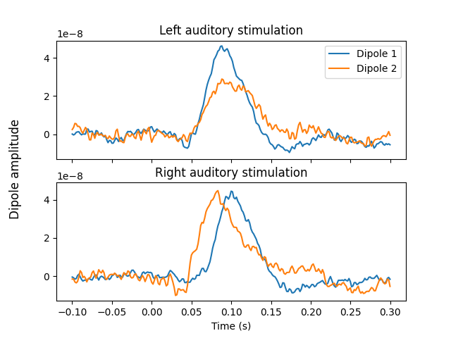
Now that we have the location and orientations of the dipoles, compute the
full timecourses using MNE, assigning activity to both dipoles at the same
time while preventing leakage between the two. We use a very low lambda
value to ensure both dipoles are fully used.
fwd, _ = mne.make_forward_dipole([dip_left, dip_right], bem, info)

# Apply MNE inverse
inv = make_inverse_operator(info, fwd, cov, fixed=True, depth=0)
stc_left = apply_inverse(evoked_left, inv, method="MNE", lambda2=1e-6)
stc_right = apply_inverse(evoked_right, inv, method="MNE", lambda2=1e-6)

# Plot the timecourses of the resulting source estimate
fig, axes = plt.subplots(nrows=2, sharex=True, sharey=True)
axes[0].plot(stc_left.times, stc_left.data.T)
axes[0].set_title("Left auditory stimulation")
axes[0].legend(["Dipole 1", "Dipole 2"])
axes[1].plot(stc_right.times, stc_right.data.T)
axes[1].set_title("Right auditory stimulation")
axes[1].set_xlabel("Time (s)")
fig.supylabel("Dipole amplitude")
Positions (in meters) and orientations
2 sources
Source space          : <SourceSpaces: [<discrete, n_used=2>] head coords, ~2 KiB>
MRI -> head transform : identity
Measurement data      : instance of Info
Conductor model   : instance of ConductorModel
Accurate field computations
Do computations in head coordinates
Free source orientations

Read 1 source spaces a total of 2 active source locations

Coordinate transformation: MRI (surface RAS) -> head
    1.000000 0.000000 0.000000       0.00 mm
    0.000000 1.000000 0.000000       0.00 mm
    0.000000 0.000000 1.000000       0.00 mm
    0.000000 0.000000 0.000000       1.00

Read 306 MEG channels from info
105 coil definitions read
Coordinate transformation: MEG device -> head
    0.991420 -0.039936 -0.124467      -6.13 mm
    0.060661 0.984012 0.167456       0.06 mm
    0.115790 -0.173570 0.977991      64.74 mm
    0.000000 0.000000 0.000000       1.00
MEG coil definitions created in head coordinates.
Source spaces are now in head coordinates.

Employing the head->MRI coordinate transform with the BEM model.
BEM model instance of ConductorModel is now set up


Source spaces are in head coordinates.
Checking that the sources are inside the surface (will take a few...)
Checking surface interior status for 2 points...
    Found 0/2 points inside  an interior sphere of radius   43.6 mm
    Found 0/2 points outside an exterior sphere of radius   91.8 mm
    Found 0/2 points outside using surface Qhull
    Found 0/2 points outside using solid angles
    Total 2/2 points inside the surface
Interior check completed in 24.6 ms
Checking surface interior status for 306 points...
    Found   0/306 points inside  an interior sphere of radius   79.1 mm
    Found   0/306 points outside an exterior sphere of radius  161.3 mm
    Found 306/306 points outside using surface Qhull
    Found   0/  0 points outside using solid angles
    Total 0/306 points inside the surface
Interior check completed in 20.6 ms

Composing the field computation matrix...
Computing MEG at 2 source locations (free orientations)...

Finished.
    Changing to fixed-orientation forward solution with surface-based source orientations...
    [done]
Computing inverse operator with 305 channels.
    305 out of 306 channels remain after picking
Selected 305 channels
Whitening the forward solution.
    Created an SSP operator (subspace dimension = 3)
Computing rank from covariance with rank=None
    Using tolerance 3.5e-13 (2.2e-16 eps * 305 dim * 5.2  max singular value)
    Estimated rank (mag + grad): 302
    MEG: rank 302 computed from 305 data channels with 3 projectors
    Setting small MEG eigenvalues to zero (without PCA)
Creating the source covariance matrix
Adjusting source covariance matrix.
Computing SVD of whitened and weighted lead field matrix.
    largest singular value = 13.9047
    scaling factor to adjust the trace = 2.18125e+16 (nchan = 305 nzero = 3)
Preparing the inverse operator for use...
    Scaled noise and source covariance from nave = 1 to nave = 65
    Created the regularized inverter
    Created an SSP operator (subspace dimension = 3)
    Created the whitener using a noise covariance matrix with rank 302 (3 small eigenvalues omitted)
Applying inverse operator to "left"...
    Picked 305 channels from the data
    Computing inverse...
    Eigenleads need to be weighted ...
    Computing residual...
    Explained  13.9% variance
[done]
Preparing the inverse operator for use...
    Scaled noise and source covariance from nave = 1 to nave = 66
    Created the regularized inverter
    Created an SSP operator (subspace dimension = 3)
    Created the whitener using a noise covariance matrix with rank 302 (3 small eigenvalues omitted)
Applying inverse operator to "right"...
    Picked 305 channels from the data
    Computing inverse...
    Eigenleads need to be weighted ...
    Computing residual...
    Explained  15.2% variance
[done]
We can also fit the timecourses to single epochs. Here, we do it for each experimental condition separately.
stcs_left = apply_inverse_epochs(epochs["left"], inv, lambda2=1e-6, method="MNE")
stcs_right = apply_inverse_epochs(epochs["right"], inv, lambda2=1e-6, method="MNE")
Preparing the inverse operator for use...
    Scaled noise and source covariance from nave = 1 to nave = 1
    Created the regularized inverter
    Created an SSP operator (subspace dimension = 3)
    Created the whitener using a noise covariance matrix with rank 302 (3 small eigenvalues omitted)
Picked 305 channels from the data
Computing inverse...
    Eigenleads need to be weighted ...
    Rejecting  epoch based on EOG : ['EOG 061']
Processing epoch : 1 / 73 (at most)
Processing epoch : 2 / 73 (at most)
Processing epoch : 3 / 73 (at most)
    Rejecting  epoch based on EOG : ['EOG 061']
Processing epoch : 4 / 73 (at most)
Processing epoch : 5 / 73 (at most)
Processing epoch : 6 / 73 (at most)
Processing epoch : 7 / 73 (at most)
Processing epoch : 8 / 73 (at most)
Processing epoch : 9 / 73 (at most)
Processing epoch : 10 / 73 (at most)
Processing epoch : 11 / 73 (at most)
Processing epoch : 12 / 73 (at most)
Processing epoch : 13 / 73 (at most)
Processing epoch : 14 / 73 (at most)
Processing epoch : 15 / 73 (at most)
Processing epoch : 16 / 73 (at most)
Processing epoch : 17 / 73 (at most)
Processing epoch : 18 / 73 (at most)
Processing epoch : 19 / 73 (at most)
Processing epoch : 20 / 73 (at most)
Processing epoch : 21 / 73 (at most)
Processing epoch : 22 / 73 (at most)
Processing epoch : 23 / 73 (at most)
Processing epoch : 24 / 73 (at most)
Processing epoch : 25 / 73 (at most)
Processing epoch : 26 / 73 (at most)
    Rejecting  epoch based on EOG : ['EOG 061']
Processing epoch : 27 / 73 (at most)
Processing epoch : 28 / 73 (at most)
Processing epoch : 29 / 73 (at most)
Processing epoch : 30 / 73 (at most)
Processing epoch : 31 / 73 (at most)
    Rejecting  epoch based on EOG : ['EOG 061']
Processing epoch : 32 / 73 (at most)
Processing epoch : 33 / 73 (at most)
Processing epoch : 34 / 73 (at most)
Processing epoch : 35 / 73 (at most)
Processing epoch : 36 / 73 (at most)
    Rejecting  epoch based on EOG : ['EOG 061']
Processing epoch : 37 / 73 (at most)
Processing epoch : 38 / 73 (at most)
Processing epoch : 39 / 73 (at most)
Processing epoch : 40 / 73 (at most)
Processing epoch : 41 / 73 (at most)
Processing epoch : 42 / 73 (at most)
    Rejecting  epoch based on EOG : ['EOG 061']
    Rejecting  epoch based on EOG : ['EOG 061']
Processing epoch : 43 / 73 (at most)
Processing epoch : 44 / 73 (at most)
Processing epoch : 45 / 73 (at most)
Processing epoch : 46 / 73 (at most)
Processing epoch : 47 / 73 (at most)
Processing epoch : 48 / 73 (at most)
Processing epoch : 49 / 73 (at most)
Processing epoch : 50 / 73 (at most)
Processing epoch : 51 / 73 (at most)
Processing epoch : 52 / 73 (at most)
    Rejecting  epoch based on EOG : ['EOG 061']
Processing epoch : 53 / 73 (at most)
Processing epoch : 54 / 73 (at most)
Processing epoch : 55 / 73 (at most)
Processing epoch : 56 / 73 (at most)
Processing epoch : 57 / 73 (at most)
Processing epoch : 58 / 73 (at most)
Processing epoch : 59 / 73 (at most)
Processing epoch : 60 / 73 (at most)
Processing epoch : 61 / 73 (at most)
Processing epoch : 62 / 73 (at most)
Processing epoch : 63 / 73 (at most)
Processing epoch : 64 / 73 (at most)
Processing epoch : 65 / 73 (at most)
[done]
Preparing the inverse operator for use...
    Scaled noise and source covariance from nave = 1 to nave = 1
    Created the regularized inverter
    Created an SSP operator (subspace dimension = 3)
    Created the whitener using a noise covariance matrix with rank 302 (3 small eigenvalues omitted)
Picked 305 channels from the data
Computing inverse...
    Eigenleads need to be weighted ...
Processing epoch : 1 / 72 (at most)
Processing epoch : 2 / 72 (at most)
Processing epoch : 3 / 72 (at most)
Processing epoch : 4 / 72 (at most)
Processing epoch : 5 / 72 (at most)
Processing epoch : 6 / 72 (at most)
Processing epoch : 7 / 72 (at most)
Processing epoch : 8 / 72 (at most)
Processing epoch : 9 / 72 (at most)
Processing epoch : 10 / 72 (at most)
Processing epoch : 11 / 72 (at most)
Processing epoch : 12 / 72 (at most)
Processing epoch : 13 / 72 (at most)
Processing epoch : 14 / 72 (at most)
Processing epoch : 15 / 72 (at most)
Processing epoch : 16 / 72 (at most)
Processing epoch : 17 / 72 (at most)
Processing epoch : 18 / 72 (at most)
Processing epoch : 19 / 72 (at most)
Processing epoch : 20 / 72 (at most)
    Rejecting  epoch based on EOG : ['EOG 061']
Processing epoch : 21 / 72 (at most)
Processing epoch : 22 / 72 (at most)
Processing epoch : 23 / 72 (at most)
Processing epoch : 24 / 72 (at most)
Processing epoch : 25 / 72 (at most)
Processing epoch : 26 / 72 (at most)
Processing epoch : 27 / 72 (at most)
    Rejecting  epoch based on MAG : ['MEG 1711']
Processing epoch : 28 / 72 (at most)
Processing epoch : 29 / 72 (at most)
Processing epoch : 30 / 72 (at most)
Processing epoch : 31 / 72 (at most)
Processing epoch : 32 / 72 (at most)
Processing epoch : 33 / 72 (at most)
Processing epoch : 34 / 72 (at most)
Processing epoch : 35 / 72 (at most)
Processing epoch : 36 / 72 (at most)
    Rejecting  epoch based on EOG : ['EOG 061']
Processing epoch : 37 / 72 (at most)
Processing epoch : 38 / 72 (at most)
    Rejecting  epoch based on EOG : ['EOG 061']
Processing epoch : 39 / 72 (at most)
Processing epoch : 40 / 72 (at most)
    Rejecting  epoch based on EOG : ['EOG 061']
Processing epoch : 41 / 72 (at most)
Processing epoch : 42 / 72 (at most)
Processing epoch : 43 / 72 (at most)
Processing epoch : 44 / 72 (at most)
Processing epoch : 45 / 72 (at most)
Processing epoch : 46 / 72 (at most)
Processing epoch : 47 / 72 (at most)
Processing epoch : 48 / 72 (at most)
Processing epoch : 49 / 72 (at most)
Processing epoch : 50 / 72 (at most)
Processing epoch : 51 / 72 (at most)
Processing epoch : 52 / 72 (at most)
Processing epoch : 53 / 72 (at most)
Processing epoch : 54 / 72 (at most)
Processing epoch : 55 / 72 (at most)
Processing epoch : 56 / 72 (at most)
Processing epoch : 57 / 72 (at most)
Processing epoch : 58 / 72 (at most)
Processing epoch : 59 / 72 (at most)
    Rejecting  epoch based on EOG : ['EOG 061']
Processing epoch : 60 / 72 (at most)
Processing epoch : 61 / 72 (at most)
Processing epoch : 62 / 72 (at most)
Processing epoch : 63 / 72 (at most)
Processing epoch : 64 / 72 (at most)
Processing epoch : 65 / 72 (at most)
Processing epoch : 66 / 72 (at most)
[done]
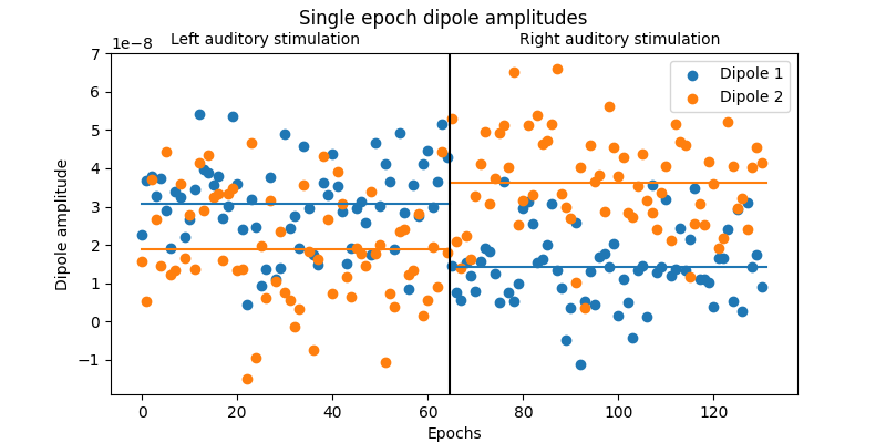
To summarize and visualize the single-epoch dipole amplitudes, we will create a detailed plot of the mean amplitude of the dipoles during different experimental conditions.
# Summarize the single epoch timecourses by computing the mean amplitude from
# 60-90ms.
amplitudes_left = []
amplitudes_right = []
for stc in stcs_left:
    amplitudes_left.append(stc.crop(0.06, 0.09).mean().data)
for stc in stcs_right:
    amplitudes_right.append(stc.crop(0.06, 0.09).mean().data)
amplitudes = np.vstack([amplitudes_left, amplitudes_right])

# Visualize the epoch-by-epoch dipole ampltudes in a detailed figure.
n = len(amplitudes)
n_left = len(amplitudes_left)
mean_left = np.mean(amplitudes_left, axis=0)
mean_right = np.mean(amplitudes_right, axis=0)

fig, ax = plt.subplots(figsize=(8, 4))
ax.scatter(np.arange(n), amplitudes[:, 0], label="Dipole 1")
ax.scatter(np.arange(n), amplitudes[:, 1], label="Dipole 2")
transition_point = n_left - 0.5
ax.plot([0, transition_point], [mean_left[0], mean_left[0]], color="C0")
ax.plot([0, transition_point], [mean_left[1], mean_left[1]], color="C1")
ax.plot([transition_point, n], [mean_right[0], mean_right[0]], color="C0")
ax.plot([transition_point, n], [mean_right[1], mean_right[1]], color="C1")
ax.axvline(transition_point, color="black")
ax.set_xlabel("Epochs")
ax.set_ylabel("Dipole amplitude")
ax.legend()
fig.suptitle("Single epoch dipole amplitudes")
fig.text(0.30, 0.9, "Left auditory stimulation", ha="center")
fig.text(0.70, 0.9, "Right auditory stimulation", ha="center")
Total running time of the script: (0 minutes 36.050 seconds)