Display sensitivity maps for EEG and MEG sensors

Sensitivity maps can be produced from forward operators that indicate how well different sensor types will be able to detect neural currents from different regions of the brain.

To get started with forward modeling see Head model and forward computation.

# Author: Eric Larson <larson.eric.d@gmail.com>
#
# License: BSD-3-Clause
# Copyright the MNE-Python contributors.

import matplotlib.pyplot as plt
import numpy as np

import mne
from mne.datasets import sample
from mne.source_estimate import SourceEstimate
from mne.source_space import compute_distance_to_sensors

print(__doc__)

data_path = sample.data_path()
meg_path = data_path / "MEG" / "sample"
fwd_fname = meg_path / "sample_audvis-meg-eeg-oct-6-fwd.fif"
subjects_dir = data_path / "subjects"

# Read the forward solutions with surface orientation
fwd = mne.read_forward_solution(fwd_fname)
mne.convert_forward_solution(fwd, surf_ori=True, copy=False)
leadfield = fwd["sol"]["data"]
print("Leadfield size : %d x %d" % leadfield.shape)

Reading forward solution from /home/circleci/mne_data/MNE-sample-data/MEG/sample/sample_audvis-meg-eeg-oct-6-fwd.fif...
    Reading a source space...
    Computing patch statistics...
    Patch information added...
    Distance information added...
    [done]
    Reading a source space...
    Computing patch statistics...
    Patch information added...
    Distance information added...
    [done]
    2 source spaces read
    Desired named matrix (kind = 3523) not available
    Read MEG forward solution (7498 sources, 306 channels, free orientations)
    Desired named matrix (kind = 3523) not available
    Read EEG forward solution (7498 sources, 60 channels, free orientations)
    Forward solutions combined: MEG, EEG
    Source spaces transformed to the forward solution coordinate frame
    Average patch normals will be employed in the rotation to the local surface coordinates....
    Converting to surface-based source orientations...
    [done]
Leadfield size : 366 x 22494

Compute sensitivity maps

grad_map = mne.sensitivity_map(fwd, ch_type="grad", mode="fixed")
mag_map = mne.sensitivity_map(fwd, ch_type="mag", mode="fixed")
eeg_map = mne.sensitivity_map(fwd, ch_type="eeg", mode="fixed")

    204 out of 366 channels remain after picking
    102 out of 366 channels remain after picking
    60 out of 366 channels remain after picking
Adding average EEG reference projection.

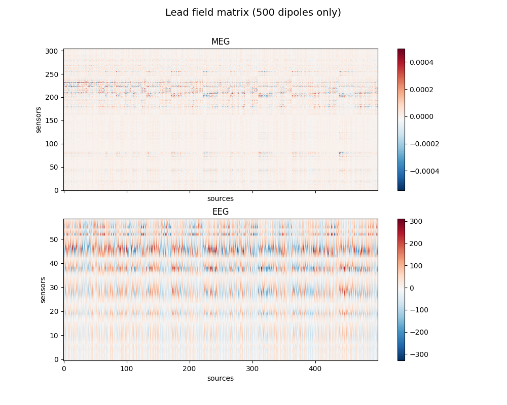
Show gain matrix a.k.a. leadfield matrix with sensitivity map

picks_meg = mne.pick_types(fwd["info"], meg=True, eeg=False)
picks_eeg = mne.pick_types(fwd["info"], meg=False, eeg=True)

fig, axes = plt.subplots(2, 1, figsize=(10, 8), sharex=True)
fig.suptitle("Lead field matrix (500 dipoles only)", fontsize=14)
for ax, picks, ch_type in zip(axes, [picks_meg, picks_eeg], ["meg", "eeg"]):
    im = ax.imshow(leadfield[picks, :500], origin="lower", aspect="auto", cmap="RdBu_r")
    ax.set_title(ch_type.upper())
    ax.set_xlabel("sources")
    ax.set_ylabel("sensors")
    fig.colorbar(im, ax=ax)

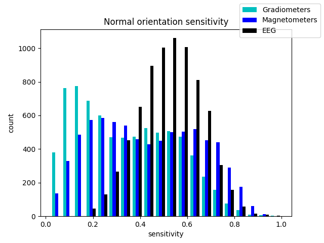
fig_2, ax = plt.subplots()
ax.hist(
    [grad_map.data.ravel(), mag_map.data.ravel(), eeg_map.data.ravel()],
    bins=20,
    label=["Gradiometers", "Magnetometers", "EEG"],
    color=["c", "b", "k"],
)
fig_2.legend()
ax.set(title="Normal orientation sensitivity", xlabel="sensitivity", ylabel="count")

brain_sens = grad_map.plot(
    subjects_dir=subjects_dir, clim=dict(lims=[0, 50, 100]), figure=1
)
brain_sens.add_text(0.1, 0.9, "Gradiometer sensitivity", "title", font_size=16)

• 
• 

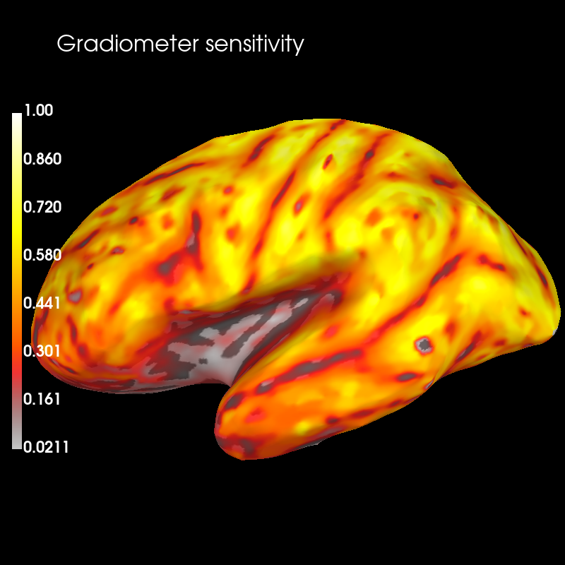
Using control points [0.02108201 0.32186553 1.        ]

Compare sensitivity map with distribution of source depths

# source space with vertices
src = fwd["src"]

# Compute minimum Euclidean distances between vertices and MEG sensors
depths = compute_distance_to_sensors(src=src, info=fwd["info"], picks=picks_meg).min(
    axis=1
)
maxdep = depths.max()  # for scaling

vertices = [src[0]["vertno"], src[1]["vertno"]]

depths_map = SourceEstimate(data=depths, vertices=vertices, tmin=0.0, tstep=1.0)

brain_dep = depths_map.plot(
    subject="sample",
    subjects_dir=subjects_dir,
    clim=dict(kind="value", lims=[0, maxdep / 2.0, maxdep]),
    figure=2,
)
brain_dep.add_text(0.1, 0.9, "Source depth (m)", "title", font_size=16)

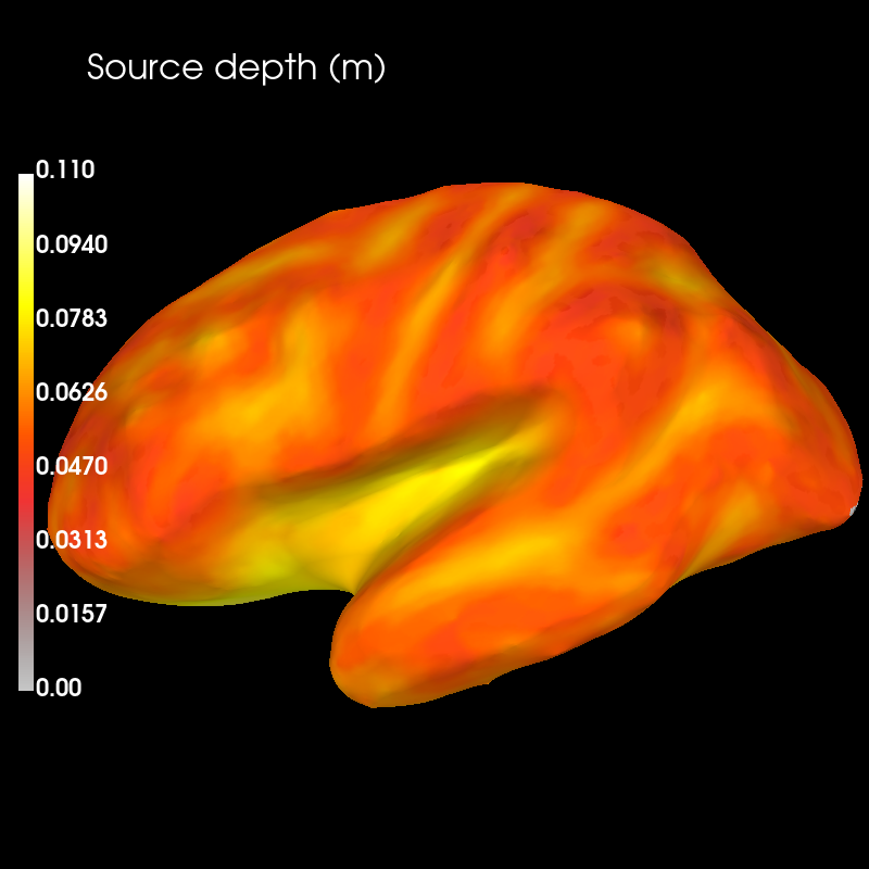
Sensitivity is likely to co-vary with the distance between sources to sensors. To determine the strength of this relationship, we can compute the correlation between source depth and sensitivity values.

corr = np.corrcoef(depths, grad_map.data[:, 0])[0, 1]
print("Correlation between source depth and gradiomter sensitivity values: %f." % corr)

Correlation between source depth and gradiomter sensitivity values: -0.815476.

Gradiometer sensitiviy is highest close to the sensors, and decreases rapidly with inreasing source depth. This is confirmed by the high negative correlation between the two.

Estimated memory usage: 225 MB