Note
Go to the end to download the full example code.
How to convert 3D electrode positions to a 2D image#
Sometimes we want to convert a 3D representation of electrodes into a 2D image. For example, if we are using electrocorticography it is common to create scatterplots on top of a brain, with each point representing an electrode.
In this example, we’ll show two ways of doing this in MNE-Python. First,
if we have the 3D locations of each electrode then we can use PyVista to
take a snapshot of a view of the brain. If we do not have these 3D locations,
and only have a 2D image of the electrodes on the brain, we can use the
mne.viz.ClickableImage class to choose our own electrode positions
on the image.
# Authors: Christopher Holdgraf <choldgraf@berkeley.edu>
#          Alex Rockhill        <aprockhill@mailbox.org>
#
# License: BSD-3-Clause
# Copyright the MNE-Python contributors.
import numpy as np
from matplotlib import pyplot as plt

import mne
from mne.io.fiff.raw import read_raw_fif
from mne.viz import (
    ClickableImage,  # noqa: F401
    plot_alignment,
    set_3d_view,
    snapshot_brain_montage,
)

misc_path = mne.datasets.misc.data_path()
subjects_dir = misc_path / "ecog"
ecog_data_fname = subjects_dir / "sample_ecog_ieeg.fif"

# We've already clicked and exported
layout_name = subjects_dir / "custom_layout.lout"
Load data#
First we will load a sample ECoG dataset which we’ll use for generating a 2D snapshot.
raw = read_raw_fif(ecog_data_fname)
raw.pick([f"G{i}" for i in range(1, 257)])  # pick just one grid

# Since we loaded in the ecog data from FIF, the coordinates
# are in 'head' space, but we actually want them in 'mri' space.
# So we will apply the head->mri transform that was used when
# generating the dataset (the estimated head->mri transform).
montage = raw.get_montage()
trans = mne.coreg.estimate_head_mri_t("sample_ecog", subjects_dir)
montage.apply_trans(trans)
Opening raw data file /home/circleci/mne_data/MNE-misc-data/ecog/sample_ecog_ieeg.fif...
    Range : 0 ... 112 =      0.000 ...     0.700 secs
Ready.
Project 3D electrodes to a 2D snapshot#
Because we have the 3D location of each electrode, we can use the
mne.viz.snapshot_brain_montage() function to return a 2D image along
with the electrode positions on that image. We use this in conjunction with
mne.viz.plot_alignment(), which visualizes electrode positions.
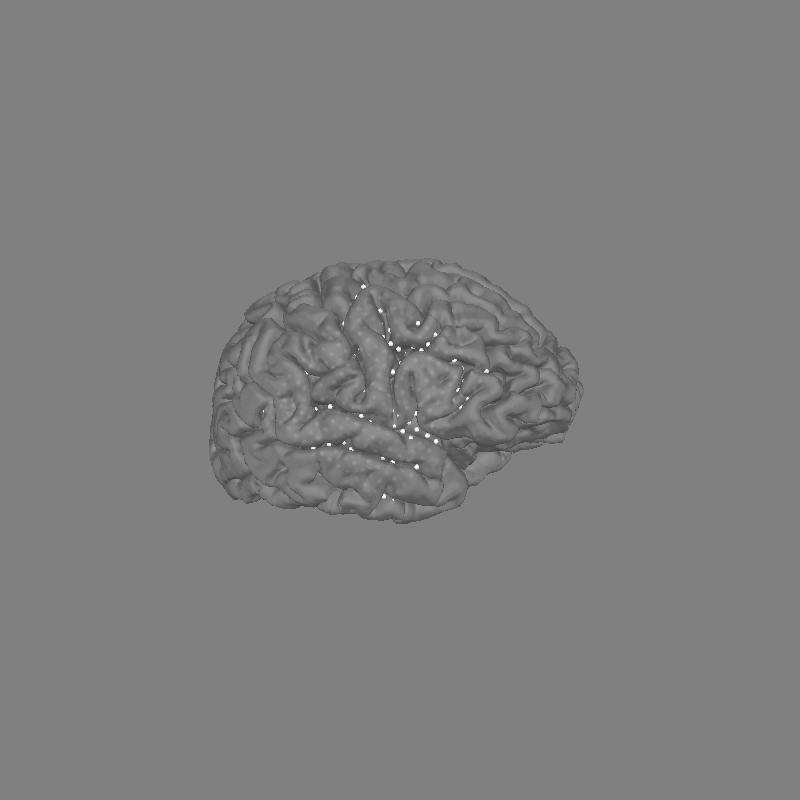
fig = plot_alignment(
raw.info,
trans=trans,
subject="sample_ecog",
subjects_dir=subjects_dir,
surfaces=dict(pial=0.9),
)
set_3d_view(figure=fig, azimuth=20, elevation=80)
xy, im = snapshot_brain_montage(fig, montage)
# Convert from a dictionary to array to plot
xy_pts = np.vstack([xy[ch] for ch in raw.ch_names])
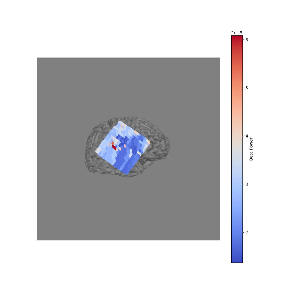
# Compute beta power to visualize
raw.load_data()
beta_power = raw.filter(20, 30).apply_hilbert(envelope=True).get_data()
beta_power = beta_power.max(axis=1) # take maximum over time
# This allows us to use matplotlib to create arbitrary 2d scatterplots
fig2, ax = plt.subplots(figsize=(10, 10))
ax.imshow(im)
cmap = ax.scatter(*xy_pts.T, c=beta_power, s=100, cmap="coolwarm")
cbar = fig2.colorbar(cmap)
cbar.ax.set_ylabel("Beta Power")
ax.set_axis_off()
# fig2.savefig('./brain.png', bbox_inches='tight') # For ClickableImage
Channel types:: ecog: 256
Reading 0 ... 112  =      0.000 ...     0.700 secs...
Filtering raw data in 1 contiguous segment
Setting up band-pass filter from 20 - 30 Hz

FIR filter parameters
---------------------
Designing a one-pass, zero-phase, non-causal bandpass filter:
- Windowed time-domain design (firwin) method
- Hamming window with 0.0194 passband ripple and 53 dB stopband attenuation
- Lower passband edge: 20.00
- Lower transition bandwidth: 5.00 Hz (-6 dB cutoff frequency: 17.50 Hz)
- Upper passband edge: 30.00 Hz
- Upper transition bandwidth: 7.50 Hz (-6 dB cutoff frequency: 33.75 Hz)
- Filter length: 107 samples (0.669 s)
Manually creating 2D electrode positions#
If we don’t have the 3D electrode positions then we can still create a
2D representation of the electrodes. Assuming that you can see the electrodes
on the 2D image, we can use mne.viz.ClickableImage to open the image
interactively. You can click points on the image and the x/y coordinate will
be stored.
We’ll open an image file, then use ClickableImage to return 2D locations of mouse clicks (or load a file already created). Then, we’ll return these xy positions as a layout for use with plotting topo maps.
# This code opens the image so you can click on it. Commented out
# because we've stored the clicks as a layout file already.

# # The click coordinates are stored as a list of tuples
# im = plt.imread('./brain.png')
# click = ClickableImage(im)
# click.plot_clicks()

# # Generate a layout from our clicks and normalize by the image
# print('Generating and saving layout...')
# lt = click.to_layout()
# lt.save(layout_name)  # save if we want

# # We've already got the layout, load it
lt = mne.channels.read_layout(layout_name, scale=False)
x = lt.pos[:, 0] * float(im.shape[1])
y = (1 - lt.pos[:, 1]) * float(im.shape[0])  # Flip the y-position
fig, ax = plt.subplots(layout="constrained")
ax.imshow(im)
ax.scatter(x, y, s=80, color="r")
ax.set_axis_off()

Total running time of the script: (0 minutes 6.768 seconds)