Note
Go to the end to download the full example code.
Source localization with equivalent current dipole (ECD) fit#
This shows how to fit a dipole [1] using MNE-Python.
For a comparison of fits between MNE-C and MNE-Python, see this gist.
# Authors: The MNE-Python contributors.
# License: BSD-3-Clause
# Copyright the MNE-Python contributors.
import matplotlib.pyplot as plt
import numpy as np
from nilearn.datasets import load_mni152_template
from nilearn.plotting import plot_anat

import mne
from mne.evoked import combine_evoked
from mne.forward import make_forward_dipole
from mne.simulation import simulate_evoked

data_path = mne.datasets.sample.data_path()
subjects_dir = data_path / "subjects"
fname_ave = data_path / "MEG" / "sample" / "sample_audvis-ave.fif"
fname_cov = data_path / "MEG" / "sample" / "sample_audvis-cov.fif"
fname_bem = subjects_dir / "sample" / "bem" / "sample-5120-bem-sol.fif"
fname_trans = data_path / "MEG" / "sample" / "sample_audvis_raw-trans.fif"
fname_surf_lh = subjects_dir / "sample" / "surf" / "lh.white"
Let’s localize the N100m (using MEG only)
evoked = mne.read_evokeds(fname_ave, condition="Right Auditory", baseline=(None, 0))
evoked.pick(picks="meg")
evoked_full = evoked.copy()
evoked.crop(0.07, 0.08)
# Fit a dipole
dip = mne.fit_dipole(evoked, fname_cov, fname_bem, fname_trans)[0]
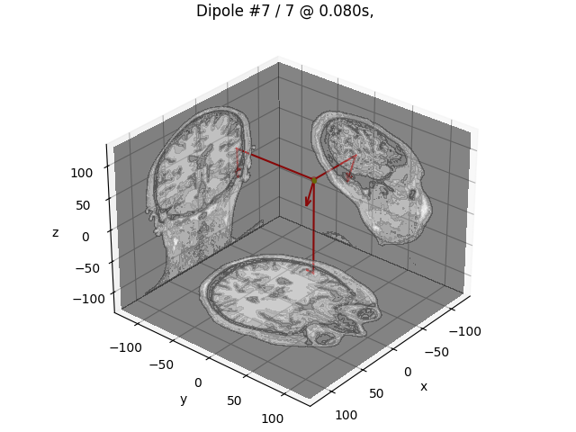
# Plot the result in 3D brain with the MRI image.
dip.plot_locations(fname_trans, "sample", subjects_dir, mode="orthoview")
Reading /home/circleci/mne_data/MNE-sample-data/MEG/sample/sample_audvis-ave.fif ...
    Read a total of 4 projection items:
        PCA-v1 (1 x 10²) active
        PCA-v2 (1 x 10²) active
        PCA-v3 (1 x 10²) active
        Average EEG reference (1 x 60) active
    Found the data of interest:
        t =    -199.80 ...     499.49 ms (Right Auditory)
        0 CTF compensation matrices available
        nave = 61 - aspect type = 100
Projections have already been applied. Setting proj attribute to True.
Applying baseline correction (mode: mean)
BEM               : PosixPath('/home/circleci/mne_data/MNE-sample-data/subjects/sample/bem/sample-5120-bem-sol.fif')
MRI transform     : /home/circleci/mne_data/MNE-sample-data/MEG/sample/sample_audvis_raw-trans.fif
Head origin       :   -4.2   19.3   65.3 mm rad =   72.3 mm.
Guess grid        :   20.0 mm
Guess mindist     :    5.0 mm
Guess exclude     :   20.0 mm
Using normal MEG coil definitions.
Noise covariance  : /home/circleci/mne_data/MNE-sample-data/MEG/sample/sample_audvis-cov.fif

Coordinate transformation: MRI (surface RAS) -> head
    0.999310 0.009985 -0.035787      -3.17 mm
    0.012759 0.812405 0.582954       6.86 mm
    0.034894 -0.583008 0.811716      28.88 mm
    0.000000 0.000000 0.000000       1.00
Coordinate transformation: MEG device -> head
    0.991420 -0.039936 -0.124467      -6.13 mm
    0.060661 0.984012 0.167456       0.06 mm
    0.115790 -0.173570 0.977991      64.74 mm
    0.000000 0.000000 0.000000       1.00
1 bad channels total
Read 305 MEG channels from info
105 coil definitions read
Coordinate transformation: MEG device -> head
    0.991420 -0.039936 -0.124467      -6.13 mm
    0.060661 0.984012 0.167456       0.06 mm
    0.115790 -0.173570 0.977991      64.74 mm
    0.000000 0.000000 0.000000       1.00
MEG coil definitions created in head coordinates.
Decomposing the sensor noise covariance matrix...
    Created an SSP operator (subspace dimension = 3)
Computing rank from covariance with rank=None
    Using tolerance 3.3e-13 (2.2e-16 eps * 305 dim * 4.8  max singular value)
    Estimated rank (mag + grad): 302
    MEG: rank 302 computed from 305 data channels with 3 projectors
    Setting small MEG eigenvalues to zero (without PCA)
    Created the whitener using a noise covariance matrix with rank 302 (3 small eigenvalues omitted)

---- Computing the forward solution for the guesses...
Guess surface (inner skull) is in MRI (surface RAS) coordinates
Filtering (grid =     20 mm)...
Surface CM = (   0.7  -10.0   44.3) mm
Surface fits inside a sphere with radius   91.8 mm
Surface extent:
    x =  -66.7 ...   68.8 mm
    y =  -88.0 ...   79.0 mm
    z =  -44.5 ...  105.8 mm
Grid extent:
    x =  -80.0 ...   80.0 mm
    y = -100.0 ...   80.0 mm
    z =  -60.0 ...  120.0 mm
900 sources before omitting any.
396 sources after omitting infeasible sources not within 20.0 - 91.8 mm.
Source spaces are in MRI coordinates.
Checking that the sources are inside the surface and at least    5.0 mm away (will take a few...)
Checking surface interior status for 396 points...
    Found  42/396 points inside  an interior sphere of radius   43.6 mm
    Found   0/396 points outside an exterior sphere of radius   91.8 mm
    Found 186/354 points outside using surface Qhull
    Found   9/168 points outside using solid angles
    Total 201/396 points inside the surface
Interior check completed in 210.6 ms
    195 source space points omitted because they are outside the inner skull surface.
    45 source space points omitted because of the    5.0-mm distance limit.
156 sources remaining after excluding the sources outside the surface and less than    5.0 mm inside.
Go through all guess source locations...
[done 156 sources]
---- Fitted :    69.9 ms, distance to inner skull : 10.6955 mm
---- Fitted :    71.6 ms, distance to inner skull : 10.6387 mm
---- Fitted :    73.3 ms, distance to inner skull : 10.5301 mm
---- Fitted :    74.9 ms, distance to inner skull : 10.2719 mm
---- Fitted :    76.6 ms, distance to inner skull : 9.9832 mm
---- Fitted :    78.3 ms, distance to inner skull : 9.7119 mm
---- Fitted :    79.9 ms, distance to inner skull : 9.4112 mm
Projections have already been applied. Setting proj attribute to True.
7 time points fitted
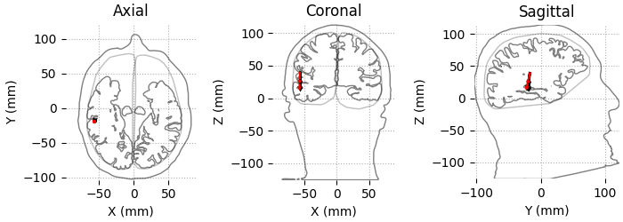
We can also plot the result using outlines of the head and brain.
color = ["k"] * len(dip)
color[np.argmax(dip.gof)] = "r"
dip.plot_locations(fname_trans, "sample", subjects_dir, mode="outlines", color=color)
Using lh.seghead for head surface.
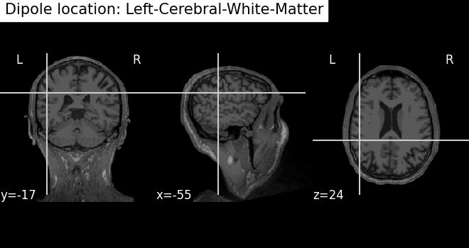
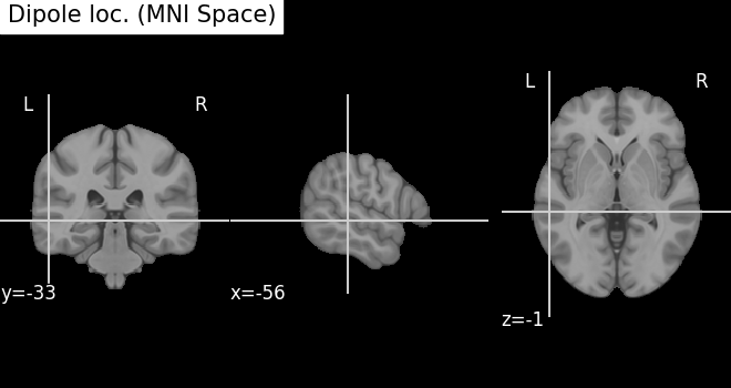
Plot the result in 3D brain with the MRI image using Nilearn In MRI coordinates and in MNI coordinates (template brain)
subject = "sample"
mni_pos = dip.to_mni(subject=subject, trans=fname_trans, subjects_dir=subjects_dir)

mri_pos = dip.to_mri(subject=subject, trans=fname_trans, subjects_dir=subjects_dir)

# Find an anatomical label for the best fitted dipole
best_dip_idx = dip.gof.argmax()
label = dip.to_volume_labels(
    fname_trans, subject=subject, subjects_dir=subjects_dir, aseg="aparc.a2009s+aseg"
)[best_dip_idx]

# Draw dipole position on MRI scan and add anatomical label from parcellation
t1_fname = subjects_dir / subject / "mri" / "T1.mgz"
fig_T1 = plot_anat(t1_fname, cut_coords=mri_pos[0], title=f"Dipole location: {label}")

try:
    template = load_mni152_template(resolution=1)
except TypeError:  # in nilearn < 0.8.1 this did not exist
    template = load_mni152_template()
fig_template = plot_anat(
    template, cut_coords=mni_pos[0], title="Dipole loc. (MNI Space)"
)
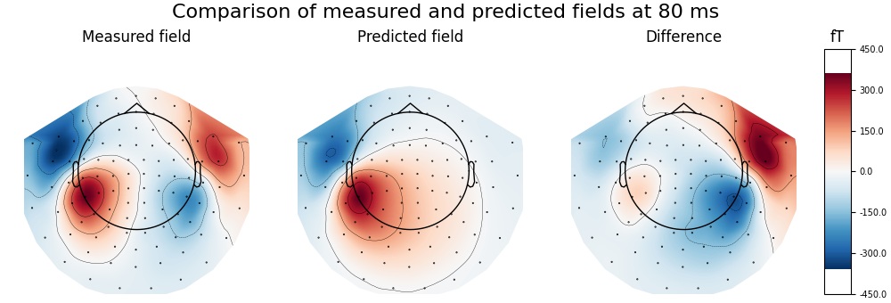
Calculate and visualise magnetic field predicted by dipole with maximum GOF and compare to the measured data, highlighting the ipsilateral (right) source
fwd, stc = make_forward_dipole(dip, fname_bem, evoked.info, fname_trans)
pred_evoked = simulate_evoked(fwd, stc, evoked.info, cov=None, nave=np.inf)

# find time point with highest GOF to plot
best_idx = np.argmax(dip.gof)
best_time = dip.times[best_idx]
print(
    f"Highest GOF {dip.gof[best_idx]:0.1f}% at t={best_time * 1000:0.1f} ms with "
    f"confidence volume {dip.conf['vol'][best_idx] * 100**3:0.1f} cm^3"
)
# remember to create a subplot for the colorbar
fig, axes = plt.subplots(
    nrows=1,
    ncols=4,
    figsize=[10.0, 3.4],
    gridspec_kw=dict(width_ratios=[1, 1, 1, 0.1], top=0.85),
    layout="constrained",
)
vmin, vmax = -400, 400  # make sure each plot has same colour range

# first plot the topography at the time of the best fitting (single) dipole
plot_params = dict(times=best_time, ch_type="mag", outlines="head", colorbar=False)
evoked.plot_topomap(time_format="Measured field", axes=axes[0], **plot_params)

# compare this to the predicted field
pred_evoked.plot_topomap(time_format="Predicted field", axes=axes[1], **plot_params)

# Subtract predicted from measured data (apply equal weights)
diff = combine_evoked([evoked, pred_evoked], weights=[1, -1])
plot_params["colorbar"] = True
diff.plot_topomap(time_format="Difference", axes=axes[2:], **plot_params)
fig.suptitle(
    f"Comparison of measured and predicted fields at {best_time * 1000:.0f} ms",
    fontsize=16,
)
Positions (in meters) and orientations
7 sources
Source space          : <SourceSpaces: [<discrete, n_used=7>] head coords, ~3 KiB>
MRI -> head transform : /home/circleci/mne_data/MNE-sample-data/MEG/sample/sample_audvis_raw-trans.fif
Measurement data      : instance of Info
Conductor model   : /home/circleci/mne_data/MNE-sample-data/subjects/sample/bem/sample-5120-bem-sol.fif
Accurate field computations
Do computations in head coordinates
Free source orientations

Read 1 source spaces a total of 7 active source locations

Coordinate transformation: MRI (surface RAS) -> head
    0.999310 0.009985 -0.035787      -3.17 mm
    0.012759 0.812405 0.582954       6.86 mm
    0.034894 -0.583008 0.811716      28.88 mm
    0.000000 0.000000 0.000000       1.00

Read 306 MEG channels from info
105 coil definitions read
Coordinate transformation: MEG device -> head
    0.991420 -0.039936 -0.124467      -6.13 mm
    0.060661 0.984012 0.167456       0.06 mm
    0.115790 -0.173570 0.977991      64.74 mm
    0.000000 0.000000 0.000000       1.00
MEG coil definitions created in head coordinates.
Source spaces are now in head coordinates.

Setting up the BEM model using /home/circleci/mne_data/MNE-sample-data/subjects/sample/bem/sample-5120-bem-sol.fif...

Loading surfaces...

Loading the solution matrix...

Homogeneous model surface loaded.
Loaded linear collocation BEM solution from /home/circleci/mne_data/MNE-sample-data/subjects/sample/bem/sample-5120-bem-sol.fif
Employing the head->MRI coordinate transform with the BEM model.
BEM model sample-5120-bem-sol.fif is now set up


Source spaces are in head coordinates.
Checking that the sources are inside the surface (will take a few...)
Checking surface interior status for 7 points...
    Found 0/7 points inside  an interior sphere of radius   43.6 mm
    Found 0/7 points outside an exterior sphere of radius   91.8 mm
    Found 0/7 points outside using surface Qhull
    Found 0/7 points outside using solid angles
    Total 7/7 points inside the surface
Interior check completed in 41.8 ms
Checking surface interior status for 306 points...
    Found   0/306 points inside  an interior sphere of radius   43.6 mm
    Found 306/306 points outside an exterior sphere of radius   91.8 mm
    Found   0/  0 points outside using surface Qhull
    Found   0/  0 points outside using solid angles
    Total 0/306 points inside the surface
Interior check completed in 27.9 ms

Composing the field computation matrix...
Computing MEG at 7 source locations (free orientations)...

Finished.
    Changing to fixed-orientation forward solution with surface-based source orientations...
    [done]
Projecting source estimate to sensor space...
[done]
Highest GOF 56.9% at t=79.9 ms with confidence volume 8.1 cm^3
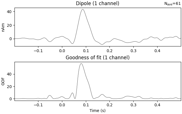
Estimate the time course of a single dipole with fixed position and orientation (the one that maximized GOF) over the entire interval
dip_fixed = mne.fit_dipole(
    evoked_full,
    fname_cov,
    fname_bem,
    fname_trans,
    pos=dip.pos[best_idx],
    ori=dip.ori[best_idx],
)[0]
dip_fixed.plot()
BEM               : PosixPath('/home/circleci/mne_data/MNE-sample-data/subjects/sample/bem/sample-5120-bem-sol.fif')
MRI transform     : /home/circleci/mne_data/MNE-sample-data/MEG/sample/sample_audvis_raw-trans.fif
Head origin       :   -4.2   19.3   65.3 mm rad =   72.3 mm.
Fixed position    :  -61.2    5.4   59.6 mm
Fixed orientation  : 0.0099 -0.7504 -0.6609 mm
Noise covariance  : /home/circleci/mne_data/MNE-sample-data/MEG/sample/sample_audvis-cov.fif

Coordinate transformation: MRI (surface RAS) -> head
    0.999310 0.009985 -0.035787      -3.17 mm
    0.012759 0.812405 0.582954       6.86 mm
    0.034894 -0.583008 0.811716      28.88 mm
    0.000000 0.000000 0.000000       1.00
Coordinate transformation: MEG device -> head
    0.991420 -0.039936 -0.124467      -6.13 mm
    0.060661 0.984012 0.167456       0.06 mm
    0.115790 -0.173570 0.977991      64.74 mm
    0.000000 0.000000 0.000000       1.00
1 bad channels total
Read 305 MEG channels from info
105 coil definitions read
Coordinate transformation: MEG device -> head
    0.991420 -0.039936 -0.124467      -6.13 mm
    0.060661 0.984012 0.167456       0.06 mm
    0.115790 -0.173570 0.977991      64.74 mm
    0.000000 0.000000 0.000000       1.00
MEG coil definitions created in head coordinates.
Decomposing the sensor noise covariance matrix...
    Created an SSP operator (subspace dimension = 3)
Computing rank from covariance with rank=None
    Using tolerance 3.3e-13 (2.2e-16 eps * 305 dim * 4.8  max singular value)
    Estimated rank (mag + grad): 302
    MEG: rank 302 computed from 305 data channels with 3 projectors
    Setting small MEG eigenvalues to zero (without PCA)
    Created the whitener using a noise covariance matrix with rank 302 (3 small eigenvalues omitted)
Compute forward for dipole location...
[done 1 source]
Projections have already been applied. Setting proj attribute to True.
421 time points fitted
References#
Total running time of the script: (0 minutes 31.710 seconds)