Note
Go to the end to download the full example code.
Optically pumped magnetometer (OPM) data#
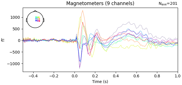
In this dataset, electrical median nerve stimulation was delivered to the left wrist of the subject. Somatosensory evoked fields were measured using nine QuSpin SERF OPMs placed over the right-hand side somatomotor area. Here we demonstrate how to localize these custom OPM data in MNE.
# Authors: The MNE-Python contributors.
# License: BSD-3-Clause
# Copyright the MNE-Python contributors.


import numpy as np

import mne

data_path = mne.datasets.opm.data_path()
subject = "OPM_sample"
subjects_dir = data_path / "subjects"
raw_fname = data_path / "MEG" / "OPM" / "OPM_SEF_raw.fif"
bem_fname = subjects_dir / subject / "bem" / f"{subject}-5120-5120-5120-bem-sol.fif"
fwd_fname = data_path / "MEG" / "OPM" / "OPM_sample-fwd.fif"
coil_def_fname = data_path / "MEG" / "OPM" / "coil_def.dat"
Prepare data for localization#
First we filter and epoch the data:
raw = mne.io.read_raw_fif(raw_fname, preload=True)
raw.filter(None, 90, h_trans_bandwidth=10.0)
raw.notch_filter(50.0, notch_widths=1)


# Set epoch rejection threshold a bit larger than for SQUIDs
reject = dict(mag=2e-10)
tmin, tmax = -0.5, 1

# Find median nerve stimulator trigger
event_id = dict(Median=257)
events = mne.find_events(raw, stim_channel="STI101", mask=257, mask_type="and")
picks = mne.pick_types(raw.info, meg=True, eeg=False)
# We use verbose='error' to suppress warning about decimation causing aliasing,
# ideally we would low-pass and then decimate instead
epochs = mne.Epochs(
    raw,
    events,
    event_id,
    tmin,
    tmax,
    verbose="error",
    reject=reject,
    picks=picks,
    proj=False,
    decim=10,
    preload=True,
)
evoked = epochs.average()
evoked.plot()
cov = mne.compute_covariance(epochs, tmax=0.0)
del epochs, raw
Opening raw data file /home/circleci/mne_data/MNE-OPM-data/MEG/OPM/OPM_SEF_raw.fif...
Isotrak not found
    Range : 0 ... 700999 =      0.000 ...   700.999 secs
Ready.
Reading 0 ... 700999  =      0.000 ...   700.999 secs...
Filtering raw data in 1 contiguous segment
Setting up low-pass filter at 90 Hz

FIR filter parameters
---------------------
Designing a one-pass, zero-phase, non-causal lowpass filter:
- Windowed time-domain design (firwin) method
- Hamming window with 0.0194 passband ripple and 53 dB stopband attenuation
- Upper passband edge: 90.00 Hz
- Upper transition bandwidth: 10.00 Hz (-6 dB cutoff frequency: 95.00 Hz)
- Filter length: 331 samples (0.331 s)

Filtering raw data in 1 contiguous segment
Setting up band-stop filter from 49 - 51 Hz

FIR filter parameters
---------------------
Designing a one-pass, zero-phase, non-causal bandstop filter:
- Windowed time-domain design (firwin) method
- Hamming window with 0.0194 passband ripple and 53 dB stopband attenuation
- Lower passband edge: 49.00
- Lower transition bandwidth: 0.50 Hz (-6 dB cutoff frequency: 48.75 Hz)
- Upper passband edge: 51.00 Hz
- Upper transition bandwidth: 0.50 Hz (-6 dB cutoff frequency: 51.25 Hz)
- Filter length: 6601 samples (6.601 s)

Finding events on: STI101
Trigger channel STI101 has a non-zero initial value of 256 (consider using initial_event=True to detect this event)
201 events found on stim channel STI101
Event IDs: [257]
Reducing data rank from 9 -> 9
Estimating covariance using EMPIRICAL
Done.
Number of samples used : 10251
[done]
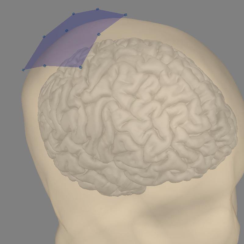
Examine our coordinate alignment for source localization and compute a forward operator:
Note
The Head<->MRI transform is an identity matrix, as the co-registration method used equates the two coordinate systems. This mis-defines the head coordinate system (which should be based on the LPA, Nasion, and RPA) but should be fine for these analyses.
bem = mne.read_bem_solution(bem_fname)
trans = mne.transforms.Transform("head", "mri")  # identity transformation

# To compute the forward solution, we must
# provide our temporary/custom coil definitions, which can be done as::
#
# with mne.use_coil_def(coil_def_fname):
#     fwd = mne.make_forward_solution(
#         raw.info, trans, src, bem, eeg=False, mindist=5.0,
#         n_jobs=None, verbose=True)

fwd = mne.read_forward_solution(fwd_fname)
# use fixed orientation here just to save memory later
mne.convert_forward_solution(fwd, force_fixed=True, copy=False)

with mne.use_coil_def(coil_def_fname):
    fig = mne.viz.plot_alignment(
        evoked.info,
        trans=trans,
        subject=subject,
        subjects_dir=subjects_dir,
        surfaces=("head", "pial"),
        bem=bem,
    )

mne.viz.set_3d_view(
    figure=fig, azimuth=45, elevation=60, distance=0.4, focalpoint=(0.02, 0, 0.04)
)
Loading surfaces...

Loading the solution matrix...

Three-layer model surfaces loaded.
Loaded linear collocation BEM solution from /home/circleci/mne_data/MNE-OPM-data/subjects/OPM_sample/bem/OPM_sample-5120-5120-5120-bem-sol.fif
Reading forward solution from /home/circleci/mne_data/MNE-OPM-data/MEG/OPM/OPM_sample-fwd.fif...
    Reading a source space...
    Computing patch statistics...
    Patch information added...
    Distance information added...
    [done]
    Reading a source space...
    Computing patch statistics...
    Patch information added...
    Distance information added...
    [done]
    2 source spaces read
    Desired named matrix (kind = 3523 (FIFF_MNE_FORWARD_SOLUTION_GRAD)) not available
    Read MEG forward solution (8196 sources, 9 channels, free orientations)
    Source spaces transformed to the forward solution coordinate frame
    Average patch normals will be employed in the rotation to the local surface coordinates....
    Converting to surface-based source orientations...
    [done]
Getting helmet for system unknown (derived from 9 MEG channel locations)
Channel types:: mag: 9
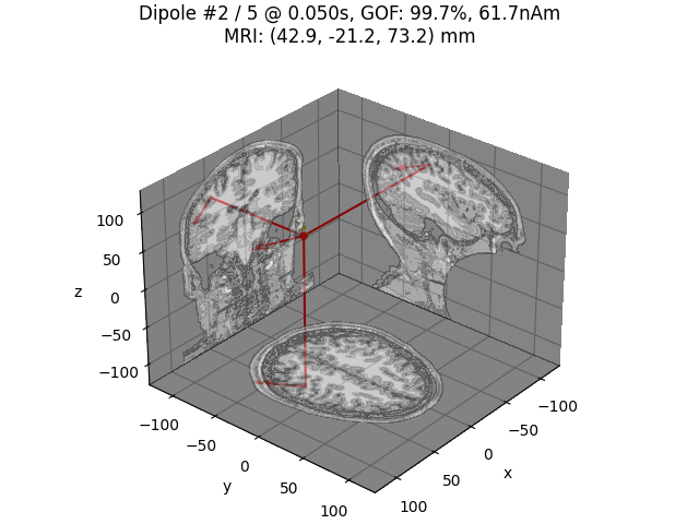
Perform dipole fitting#
# Fit dipoles on a subset of time points
with mne.use_coil_def(coil_def_fname):
    dip_opm, _ = mne.fit_dipole(
        evoked.copy().crop(0.040, 0.080), cov, bem, trans, verbose=True
    )
idx = np.argmax(dip_opm.gof)
print(
    f"Best dipole at t={1000 * dip_opm.times[idx]:0.1f} ms with "
    f"{dip_opm.gof[idx]:0.1f}% GOF"
)

# Plot N20m dipole as an example
dip_opm.plot_locations(trans, subject, subjects_dir, mode="orthoview", idx=idx)
BEM               : <ConductorModel | BEM (3 layers) solver=mne>
MRI transform     : instance of Transform
Head origin       :    1.3  -14.2   35.5 mm rad =   78.4 mm.
Guess grid        :   20.0 mm
Guess mindist     :    5.0 mm
Guess exclude     :   20.0 mm
Using normal MEG coil definitions.
Noise covariance  : <Covariance | kind : full, shape : (9, 9), range : [+5.2e-26, +2.4e-25], n_samples : 10250>

Coordinate transformation: MRI (surface RAS) -> head
    1.000000 0.000000 0.000000       0.00 mm
    0.000000 1.000000 0.000000       0.00 mm
    0.000000 0.000000 1.000000       0.00 mm
    0.000000 0.000000 0.000000       1.00
Coordinate transformation: MEG device -> head
    0.999800 0.015800 -0.009200       0.10 mm
    -0.018100 0.930500 -0.365900      16.60 mm
    0.002800 0.366000 0.930600     -14.40 mm
    0.000000 0.000000 0.000000       1.00
0 bad channels total
Read 9 MEG channels from info
2 coil definitions read
105 coil definitions read
Coordinate transformation: MEG device -> head
    0.999800 0.015800 -0.009200       0.10 mm
    -0.018100 0.930500 -0.365900      16.60 mm
    0.002800 0.366000 0.930600     -14.40 mm
    0.000000 0.000000 0.000000       1.00
MEG coil definitions created in head coordinates.
Decomposing the sensor noise covariance matrix...
Computing rank from covariance with rank=None
    Using tolerance 2.2e-15 (2.2e-16 eps * 9 dim * 1.1  max singular value)
    Estimated rank (mag): 9
    MAG: rank 9 computed from 9 data channels with 0 projectors
    Setting small MAG eigenvalues to zero (without PCA)
    Created the whitener using a noise covariance matrix with rank 9 (0 small eigenvalues omitted)

---- Computing the forward solution for the guesses...
Guess surface (inner skull) is in MRI (surface RAS) coordinates
Filtering (grid =     20 mm)...
Surface CM = (   1.5  -15.0   35.4) mm
Surface fits inside a sphere with radius  102.1 mm
Surface extent:
    x =  -73.3 ...   77.3 mm
    y = -100.7 ...   86.4 mm
    z =  -42.9 ...  108.2 mm
Grid extent:
    x =  -80.0 ...   80.0 mm
    y = -120.0 ...  100.0 mm
    z =  -60.0 ...  120.0 mm
1080 sources before omitting any.
543 sources after omitting infeasible sources not within 20.0 - 102.1 mm.
Source spaces are in MRI coordinates.
Checking that the sources are inside the surface and at least    5.0 mm away (will take a few...)
Checking surface interior status for 543 points...
    Found  70/543 points inside  an interior sphere of radius   51.5 mm
    Found   0/543 points outside an exterior sphere of radius  102.1 mm
    Found 284/473 points outside using surface Qhull
    Found  15/189 points outside using solid angles
    Total 244/543 points inside the surface
Interior check completed in 250.4 ms
    299 source space points omitted because they are outside the inner skull surface.
    30 source space points omitted because of the    5.0-mm distance limit.
214 sources remaining after excluding the sources outside the surface and less than    5.0 mm inside.
Go through all guess source locations...
[done 214 sources]
---- Fitted :    40.0 ms, distance to inner skull : 9.2421 mm
---- Fitted :    50.0 ms, distance to inner skull : 15.2879 mm
---- Fitted :    60.0 ms, distance to inner skull : 18.8049 mm
---- Fitted :    70.0 ms, distance to inner skull : 14.7042 mm
---- Fitted :    80.0 ms, distance to inner skull : 5.2171 mm
No projector specified for this dataset. Please consider the method self.add_proj.
5 time points fitted
Best dipole at t=50.0 ms with 99.7% GOF
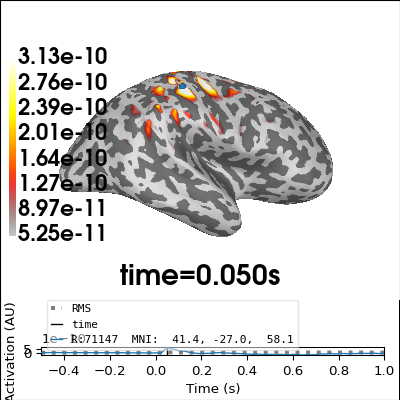
Perform minimum-norm localization#
Due to the small number of sensors, there will be some leakage of activity to areas with low/no sensitivity. Constraining the source space to areas we are sensitive to might be a good idea.
inverse_operator = mne.minimum_norm.make_inverse_operator(
    evoked.info, fwd, cov, loose=0.0, depth=None
)
del fwd, cov

method = "MNE"
snr = 3.0
lambda2 = 1.0 / snr**2
stc = mne.minimum_norm.apply_inverse(
    evoked, inverse_operator, lambda2, method=method, pick_ori=None, verbose=True
)

# Plot source estimate at time of best dipole fit
brain = stc.plot(
    hemi="rh",
    views="lat",
    subjects_dir=subjects_dir,
    initial_time=dip_opm.times[idx],
    clim=dict(kind="percent", lims=[99, 99.9, 99.99]),
    size=(800, 600),
    background="w",
)
Computing inverse operator with 9 channels.
    9 out of 9 channels remain after picking
Selected 9 channels
Whitening the forward solution.
Computing rank from covariance with rank=None
    Using tolerance 2.2e-15 (2.2e-16 eps * 9 dim * 1.1  max singular value)
    Estimated rank (mag): 9
    MAG: rank 9 computed from 9 data channels with 0 projectors
    Setting small MAG eigenvalues to zero (without PCA)
Creating the source covariance matrix
Adjusting source covariance matrix.
Computing SVD of whitened and weighted lead field matrix.
    largest singular value = 1.38802
    scaling factor to adjust the trace = 7.35945e+18 (nchan = 9 nzero = 0)
Preparing the inverse operator for use...
    Scaled noise and source covariance from nave = 1 to nave = 201
    Created the regularized inverter
    The projection vectors do not apply to these channels.
    Created the whitener using a noise covariance matrix with rank 9 (0 small eigenvalues omitted)
Applying inverse operator to "Median"...
    Picked 9 channels from the data
    Computing inverse...
    Eigenleads need to be weighted ...
    Computing residual...
    Explained  97.7% variance
[done]
Using control points [5.24807258e-11 1.55793898e-10 3.13115753e-10]
Total running time of the script: (0 minutes 21.597 seconds)