Note
Go to the end to download the full example code.
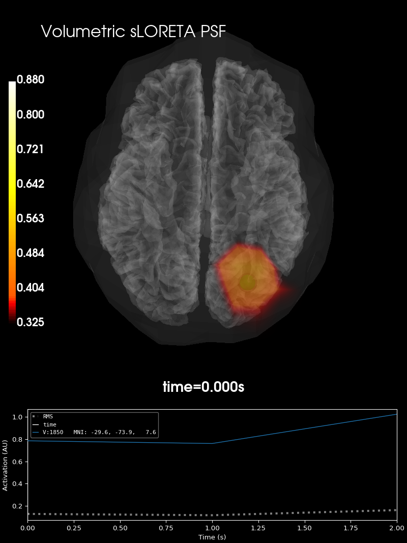
Plot point-spread functions (PSFs) for a volume#
Visualise PSF at one volume vertex for sLORETA.
# Authors: Olaf Hauk <olaf.hauk@mrc-cbu.cam.ac.uk>
#          Alexandre Gramfort <alexandre.gramfort@inria.fr>
#          Eric Larson <larson.eric.d@gmail.com>
#
# License: BSD-3-Clause
# Copyright the MNE-Python contributors.
import numpy as np

import mne
from mne.datasets import sample
from mne.minimum_norm import get_point_spread, make_inverse_resolution_matrix

print(__doc__)

data_path = sample.data_path()
subjects_dir = data_path / "subjects"
meg_path = data_path / "MEG" / "sample"
fname_cov = meg_path / "sample_audvis-cov.fif"
fname_evo = meg_path / "sample_audvis-ave.fif"
fname_trans = meg_path / "sample_audvis_raw-trans.fif"
fname_bem = subjects_dir / "sample" / "bem" / "sample-5120-bem-sol.fif"
For the volume, create a coarse source space for speed (don’t do this in real code!), then compute the forward using this source space.
# read noise cov and and evoked
noise_cov = mne.read_cov(fname_cov)
evoked = mne.read_evokeds(fname_evo, 0)

# create a coarse source space
src_vol = mne.setup_volume_source_space(  # this is a very course resolution!
    "sample", pos=15.0, subjects_dir=subjects_dir, add_interpolator=False
)  # usually you want True, this is just for speed

# compute the forward
forward_vol = mne.make_forward_solution(  # MEG-only for speed
    evoked.info, fname_trans, src_vol, fname_bem, eeg=False
)
del src_vol
    366 x 366 full covariance (kind = 1) found.
    Read a total of 4 projection items:
        PCA-v1 (1 x 10²) active
        PCA-v2 (1 x 10²) active
        PCA-v3 (1 x 10²) active
        Average EEG reference (1 x 60) active
Reading /home/circleci/mne_data/MNE-sample-data/MEG/sample/sample_audvis-ave.fif ...
    Read a total of 4 projection items:
        PCA-v1 (1 x 10²) active
        PCA-v2 (1 x 10²) active
        PCA-v3 (1 x 10²) active
        Average EEG reference (1 x 60) active
    Found the data of interest:
        t =    -199.80 ...     499.49 ms (Left Auditory)
        0 CTF compensation matrices available
        nave = 55 - aspect type = 100
Projections have already been applied. Setting proj attribute to True.
No baseline correction applied
Sphere                : origin at (0.0 0.0 0.0) mm
              radius  : 95.0 mm
grid                  : 15.0 mm
mindist               : 5.0 mm
MRI volume            : /home/circleci/mne_data/MNE-sample-data/subjects/sample/mri/T1.mgz

Reading /home/circleci/mne_data/MNE-sample-data/subjects/sample/mri/T1.mgz...

Setting up the sphere...
Surface CM = (   0.0    0.0    0.0) mm
Surface fits inside a sphere with radius   95.0 mm
Surface extent:
    x =  -95.0 ...   95.0 mm
    y =  -95.0 ...   95.0 mm
    z =  -95.0 ...   95.0 mm
Grid extent:
    x = -105.0 ...  105.0 mm
    y = -105.0 ...  105.0 mm
    z = -105.0 ...  105.0 mm
3375 sources before omitting any.
1045 sources after omitting infeasible sources not within 0.0 - 95.0 mm.
Source spaces are in MRI coordinates.
Checking that the sources are inside the surface and at least    5.0 mm away (will take a few...)
    120 source space point omitted because of the    5.0-mm distance limit.
925 sources remaining after excluding the sources outside the surface and less than    5.0 mm inside.
Adjusting the neighborhood info.
Source space : MRI voxel -> MRI (surface RAS)
    0.015000 0.000000 0.000000    -105.00 mm
    0.000000 0.015000 0.000000    -105.00 mm
    0.000000 0.000000 0.015000    -105.00 mm
    0.000000 0.000000 0.000000       1.00
MRI volume : MRI voxel -> MRI (surface RAS)
    -0.001000 0.000000 0.000000     128.00 mm
    0.000000 0.000000 0.001000    -128.00 mm
    0.000000 -0.001000 0.000000     128.00 mm
    0.000000 0.000000 0.000000       1.00
MRI volume : MRI (surface RAS) -> RAS (non-zero origin)
    1.000000 -0.000000 -0.000000      -5.27 mm
    -0.000000 1.000000 -0.000000       9.04 mm
    -0.000000 0.000000 1.000000     -27.29 mm
    0.000000 0.000000 0.000000       1.00
Source space          : <SourceSpaces: [<volume, shape=(np.int64(15), np.int64(15), np.int64(15)), n_used=925>] MRI (surface RAS) coords, subject 'sample', ~859 KiB>
MRI -> head transform : /home/circleci/mne_data/MNE-sample-data/MEG/sample/sample_audvis_raw-trans.fif
Measurement data      : instance of Info
Conductor model   : /home/circleci/mne_data/MNE-sample-data/subjects/sample/bem/sample-5120-bem-sol.fif
Accurate field computations
Do computations in head coordinates
Free source orientations

Read 1 source spaces a total of 925 active source locations

Coordinate transformation: MRI (surface RAS) -> head
    0.999310 0.009985 -0.035787      -3.17 mm
    0.012759 0.812405 0.582954       6.86 mm
    0.034894 -0.583008 0.811716      28.88 mm
    0.000000 0.000000 0.000000       1.00

Read 306 MEG channels from info
105 coil definitions read
Coordinate transformation: MEG device -> head
    0.991420 -0.039936 -0.124467      -6.13 mm
    0.060661 0.984012 0.167456       0.06 mm
    0.115790 -0.173570 0.977991      64.74 mm
    0.000000 0.000000 0.000000       1.00
MEG coil definitions created in head coordinates.
Source spaces are now in head coordinates.

Setting up the BEM model using /home/circleci/mne_data/MNE-sample-data/subjects/sample/bem/sample-5120-bem-sol.fif...

Loading surfaces...

Loading the solution matrix...

Homogeneous model surface loaded.
Loaded linear collocation BEM solution from /home/circleci/mne_data/MNE-sample-data/subjects/sample/bem/sample-5120-bem-sol.fif
Employing the head->MRI coordinate transform with the BEM model.
BEM model sample-5120-bem-sol.fif is now set up


Source spaces are in head coordinates.
Checking that the sources are inside the surface (will take a few...)
Checking surface interior status for 925 points...
    Found 103/925 points inside  an interior sphere of radius   43.6 mm
    Found 322/925 points outside an exterior sphere of radius   91.8 mm
    Found 163/500 points outside using surface Qhull
    Found  30/337 points outside using solid angles
    Total 410/925 points inside the surface
Interior check completed in 55.0 ms
    515 source space points omitted because they are outside the inner skull surface.
Checking surface interior status for 306 points...
    Found   0/306 points inside  an interior sphere of radius   43.6 mm
    Found 306/306 points outside an exterior sphere of radius   91.8 mm
    Found   0/  0 points outside using surface Qhull
    Found   0/  0 points outside using solid angles
    Total 0/306 points inside the surface
Interior check completed in 1.1 ms

Composing the field computation matrix...
Computing MEG at 410 source locations (free orientations)...

Finished.
Now make an inverse operator and compute the PSF at a source.
inverse_operator_vol = mne.minimum_norm.make_inverse_operator(
    info=evoked.info, forward=forward_vol, noise_cov=noise_cov
)

# compute resolution matrix for sLORETA
rm_lor_vol = make_inverse_resolution_matrix(
    forward_vol, inverse_operator_vol, method="sLORETA", lambda2=1.0 / 9.0
)

# get PSF and CTF for sLORETA at one vertex
sources_vol = [100]
stc_psf_vol = get_point_spread(rm_lor_vol, forward_vol["src"], sources_vol, norm=True)
del rm_lor_vol
Computing inverse operator with 305 channels.
    305 out of 306 channels remain after picking
Selected 305 channels
Creating the depth weighting matrix...
    203 planar channels
    limit = 390/410 = 10.140193
    scale = 3.7904e-08 exp = 0.8
Whitening the forward solution.
    Created an SSP operator (subspace dimension = 3)
Computing rank from covariance with rank=None
    Using tolerance 3.3e-13 (2.2e-16 eps * 305 dim * 4.8  max singular value)
    Estimated rank (mag + grad): 302
    MEG: rank 302 computed from 305 data channels with 3 projectors
    Setting small MEG eigenvalues to zero (without PCA)
Creating the source covariance matrix
Adjusting source covariance matrix.
Computing SVD of whitened and weighted lead field matrix.
    largest singular value = 4.60207
    scaling factor to adjust the trace = 1.36129e+18 (nchan = 305 nzero = 3)
    305 out of 306 channels remain after picking
Preparing the inverse operator for use...
    Scaled noise and source covariance from nave = 1 to nave = 1
    Created the regularized inverter
    Created an SSP operator (subspace dimension = 3)
    Created the whitener using a noise covariance matrix with rank 302 (3 small eigenvalues omitted)
    Computing noise-normalization factors (sLORETA)...
[done]
Applying inverse operator to ""...
    Picked 305 channels from the data
    Computing inverse...
    Eigenleads need to be weighted ...
    Computing residual...
    Explained  46.0% variance
    sLORETA...
[done]
Dimension of Inverse Matrix: (1230, 305)
Dimensions of resolution matrix: 1230 by 1230.
Visualize#
PSF:
# Which vertex corresponds to selected source
src_vol = forward_vol["src"]
verttrue_vol = src_vol[0]["vertno"][sources_vol]

# find vertex with maximum in PSF
max_vert_idx, _ = np.unravel_index(stc_psf_vol.data.argmax(), stc_psf_vol.data.shape)
vert_max_ctf_vol = src_vol[0]["vertno"][[max_vert_idx]]

# plot them
brain_psf_vol = stc_psf_vol.plot_3d(
    "sample",
    src=forward_vol["src"],
    views="ven",
    subjects_dir=subjects_dir,
    volume_options=dict(alpha=0.5, interpolation="nearest", silhouette_alpha=0.5),
)
brain_psf_vol.add_text(0.1, 0.9, "Volumetric sLORETA PSF", "title", font_size=16)
brain_psf_vol.add_foci(
    verttrue_vol, coords_as_verts=True, scale_factor=1, hemi="vol", color="green"
)
brain_psf_vol.add_foci(
    vert_max_ctf_vol,
    coords_as_verts=True,
    scale_factor=1.25,
    hemi="vol",
    color="black",
    alpha=0.3,
)
Using control points [0.32037612 0.38043126 0.87946273]
Total running time of the script: (0 minutes 24.826 seconds)