2 samples permutation test on source data with spatio-temporal clustering

Tests if the source space data are significantly different between 2 groups of subjects (simulated here using one subject’s data). The multiple comparisons problem is addressed with a cluster-level permutation test across space and time.

# Authors: Alexandre Gramfort <alexandre.gramfort@inria.fr>
#          Eric Larson <larson.eric.d@gmail.com>
# License: BSD-3-Clause
# Copyright the MNE-Python contributors.

import numpy as np
from scipy import stats as stats

import mne
from mne import spatial_src_adjacency
from mne.datasets import sample
from mne.stats import spatio_temporal_cluster_test, summarize_clusters_stc

print(__doc__)

Set parameters

data_path = sample.data_path()
meg_path = data_path / "MEG" / "sample"
stc_fname = meg_path / "sample_audvis-meg-lh.stc"
subjects_dir = data_path / "subjects"
src_fname = subjects_dir / "fsaverage" / "bem" / "fsaverage-ico-5-src.fif"

# Load stc to in common cortical space (fsaverage)
stc = mne.read_source_estimate(stc_fname)
stc.resample(50, npad="auto")

# Read the source space we are morphing to
src = mne.read_source_spaces(src_fname)
fsave_vertices = [s["vertno"] for s in src]
morph = mne.compute_source_morph(
    stc,
    "sample",
    "fsaverage",
    spacing=fsave_vertices,
    smooth=20,
    subjects_dir=subjects_dir,
)
stc = morph.apply(stc)
n_vertices_fsave, n_times = stc.data.shape
tstep = stc.tstep * 1000  # convert to milliseconds

n_subjects1, n_subjects2 = 6, 7
print(f"Simulating data for {n_subjects1} and {n_subjects2} subjects.")

#    Let's make sure our results replicate, so set the seed.
np.random.seed(0)
X1 = np.random.randn(n_vertices_fsave, n_times, n_subjects1) * 10
X2 = np.random.randn(n_vertices_fsave, n_times, n_subjects2) * 10
X1[:, :, :] += stc.data[:, :, np.newaxis]
# make the activity bigger for the second set of subjects
X2[:, :, :] += 3 * stc.data[:, :, np.newaxis]

#    We want to compare the overall activity levels for each subject
X1 = np.abs(X1)  # only magnitude
X2 = np.abs(X2)  # only magnitude

    Reading a source space...
    [done]
    Reading a source space...
    [done]
    2 source spaces read
surface source space present ...
Computing morph matrix...
    Left-hemisphere map read.
    Right-hemisphere map read.
    20 smooth iterations done.
    20 smooth iterations done.
[done]
[done]
Simulating data for 6 and 7 subjects.

Compute statistic

To use an algorithm optimized for spatio-temporal clustering, we just pass the spatial adjacency matrix (instead of spatio-temporal)

print("Computing adjacency.")
adjacency = spatial_src_adjacency(src)

#    Note that X needs to be a list of multi-dimensional array of shape
#    samples (subjects_k) × time × space, so we permute dimensions
X1 = np.transpose(X1, [2, 1, 0])
X2 = np.transpose(X2, [2, 1, 0])
X = [X1, X2]

# Now let's actually do the clustering. This can take a long time...
# Here we set the threshold quite high to reduce computation,
# and use a very low number of permutations for the same reason.
n_permutations = 50
p_threshold = 0.001
f_threshold = stats.distributions.f.ppf(
    1.0 - p_threshold / 2.0, n_subjects1 - 1, n_subjects2 - 1
)
print("Clustering.")
F_obs, clusters, cluster_p_values, H0 = clu = spatio_temporal_cluster_test(
    X,
    adjacency=adjacency,
    n_jobs=None,
    n_permutations=n_permutations,
    threshold=f_threshold,
    buffer_size=None,
)
#    Now select the clusters that are sig. at p < 0.05 (note that this value
#    is multiple-comparisons corrected).
good_cluster_inds = np.where(cluster_p_values < 0.05)[0]

Computing adjacency.
-- number of adjacent vertices : 20484
Clustering.
stat_fun(H1): min=1.8724146338349605e-13 max=303.63217183709247
Running initial clustering …
Found 361 clusters

  0%|          | Permuting : 0/49 [00:00<?,       ?it/s]
  2%|▏         | Permuting : 1/49 [00:00<00:01,   29.59it/s]
  6%|▌         | Permuting : 3/49 [00:00<00:01,   44.80it/s]
 10%|█         | Permuting : 5/49 [00:00<00:00,   49.85it/s]
 12%|█▏        | Permuting : 6/49 [00:00<00:00,   44.40it/s]
 16%|█▋        | Permuting : 8/49 [00:00<00:00,   47.71it/s]
 20%|██        | Permuting : 10/49 [00:00<00:00,   49.91it/s]
 24%|██▍       | Permuting : 12/49 [00:00<00:00,   51.47it/s]
 29%|██▊       | Permuting : 14/49 [00:00<00:00,   52.08it/s]
 33%|███▎      | Permuting : 16/49 [00:00<00:00,   46.46it/s]
 35%|███▍      | Permuting : 17/49 [00:00<00:00,   44.60it/s]
 39%|███▉      | Permuting : 19/49 [00:00<00:00,   46.12it/s]
 41%|████      | Permuting : 20/49 [00:00<00:00,   44.49it/s]
 45%|████▍     | Permuting : 22/49 [00:00<00:00,   45.70it/s]
 49%|████▉     | Permuting : 24/49 [00:00<00:00,   46.92it/s]
 51%|█████     | Permuting : 25/49 [00:00<00:00,   45.44it/s]
 55%|█████▌    | Permuting : 27/49 [00:00<00:00,   46.57it/s]
 57%|█████▋    | Permuting : 28/49 [00:00<00:00,   45.15it/s]
 61%|██████    | Permuting : 30/49 [00:00<00:00,   45.96it/s]
 65%|██████▌   | Permuting : 32/49 [00:00<00:00,   46.97it/s]
 69%|██████▉   | Permuting : 34/49 [00:00<00:00,   47.89it/s]
 71%|███████▏  | Permuting : 35/49 [00:00<00:00,   46.58it/s]
 73%|███████▎  | Permuting : 36/49 [00:00<00:00,   45.40it/s]
 78%|███████▊  | Permuting : 38/49 [00:00<00:00,   46.11it/s]
 82%|████████▏ | Permuting : 40/49 [00:00<00:00,   46.88it/s]
 84%|████████▎ | Permuting : 41/49 [00:00<00:00,   45.75it/s]
 88%|████████▊ | Permuting : 43/49 [00:00<00:00,   46.40it/s]
 90%|████████▉ | Permuting : 44/49 [00:00<00:00,   45.34it/s]
 94%|█████████▍| Permuting : 46/49 [00:00<00:00,   46.22it/s]
 96%|█████████▌| Permuting : 47/49 [00:01<00:00,   45.19it/s]
100%|██████████| Permuting : 49/49 [00:01<00:00,   46.59it/s]
100%|██████████| Permuting : 49/49 [00:01<00:00,   46.45it/s]

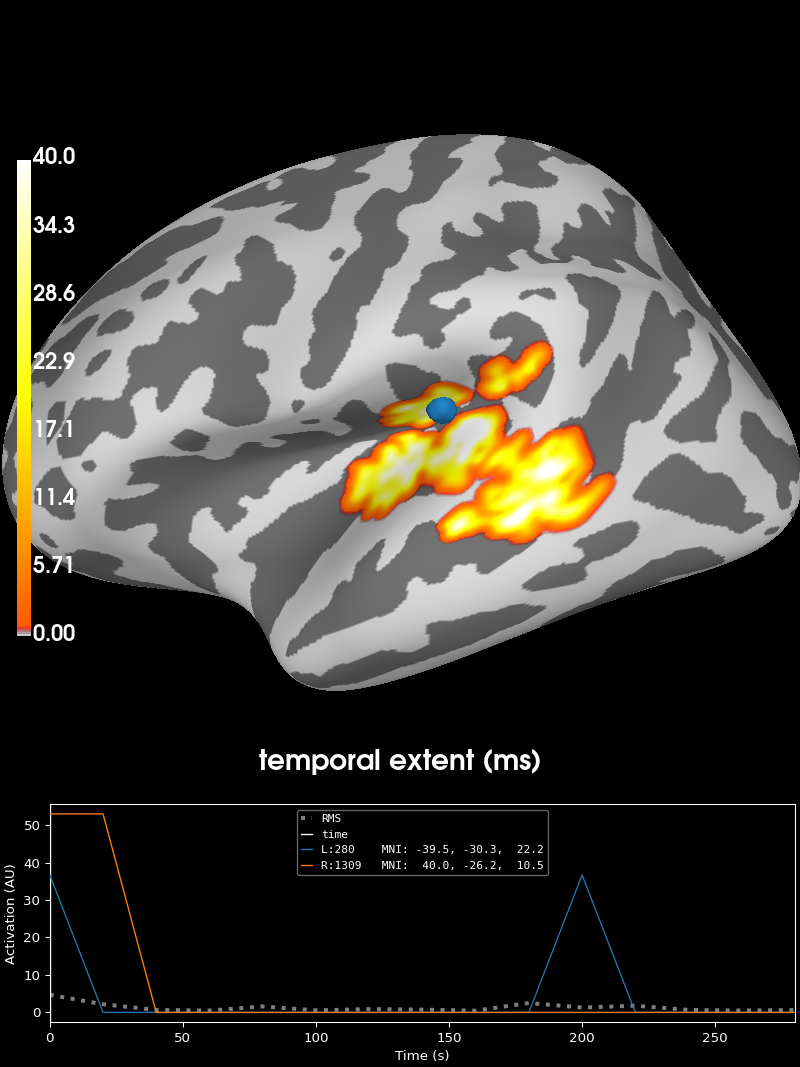
Visualize the clusters

print("Visualizing clusters.")

#    Now let's build a convenient representation of each cluster, where each
#    cluster becomes a "time point" in the SourceEstimate
fsave_vertices = [np.arange(10242), np.arange(10242)]
stc_all_cluster_vis = summarize_clusters_stc(
    clu, tstep=tstep, vertices=fsave_vertices, subject="fsaverage"
)

#    Let's actually plot the first "time point" in the SourceEstimate, which
#    shows all the clusters, weighted by duration

# blue blobs are for condition A != condition B
brain = stc_all_cluster_vis.plot(
    "fsaverage",
    hemi="both",
    views="lateral",
    subjects_dir=subjects_dir,
    time_label="temporal extent (ms)",
    clim=dict(kind="value", lims=[0, 1, 40]),
)

Visualizing clusters.
True