Note
Go to the end to download the full example code.
Auto-generating Epochs metadata#
This tutorial shows how to auto-generate metadata for Epochs, based on
events via mne.epochs.make_metadata.
We are going to use data from the ERP CORE Dataset (derived from [1]). This is EEG data from a single participant performing an active visual task (Eriksen flanker task).
Note
If you wish to skip the introductory parts of this tutorial, you may jump straight to Applying the knowledge: visualizing the ERN component after completing the data import and event creation in the Preparation section.
This tutorial is loosely divided into two parts:
We will first focus on producing ERPs time-locked to the visual stimulation, conditional on response correctness and response time in order to familiarize ourselves with the
make_metadatafunction.After that, we will calculate ERPs time-locked to the responses – again, conditional on response correctness – to visualize the error-related negativity (ERN), i.e. the ERP component associated with incorrect behavioral responses.
Preparation#
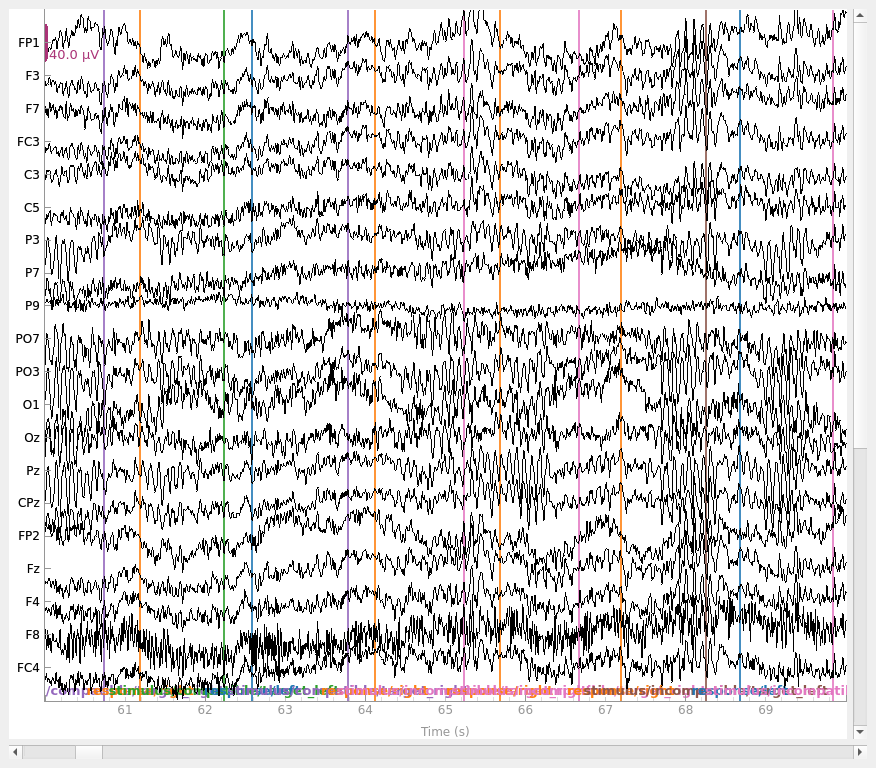
Let’s start by reading, filtering, and producing a simple visualization of the
raw data. The data is pretty clean and contains very few blinks, so there’s no
need to apply sophisticated preprocessing and data cleaning procedures.
We will also convert the Annotations contained in this dataset to events
by calling mne.events_from_annotations.
# Authors: Richard Höchenberger <richard.hoechenberger@gmail.com>
# License: BSD-3-Clause
# Copyright the MNE-Python contributors.
import matplotlib.pyplot as plt

import mne

data_dir = mne.datasets.erp_core.data_path()
infile = data_dir / "ERP-CORE_Subject-001_Task-Flankers_eeg.fif"

raw = mne.io.read_raw(infile, preload=True)
raw.filter(l_freq=0.1, h_freq=40)
raw.plot(start=60)

# extract events
all_events, all_event_id = mne.events_from_annotations(raw)
Opening raw data file /home/circleci/mne_data/MNE-ERP-CORE-data/ERP-CORE_Subject-001_Task-Flankers_eeg.fif...
    Range : 0 ... 935935 =      0.000 ...   913.999 secs
Ready.
Reading 0 ... 935935  =      0.000 ...   913.999 secs...
Filtering raw data in 1 contiguous segment
Setting up band-pass filter from 0.1 - 40 Hz

FIR filter parameters
---------------------
Designing a one-pass, zero-phase, non-causal bandpass filter:
- Windowed time-domain design (firwin) method
- Hamming window with 0.0194 passband ripple and 53 dB stopband attenuation
- Lower passband edge: 0.10
- Lower transition bandwidth: 0.10 Hz (-6 dB cutoff frequency: 0.05 Hz)
- Upper passband edge: 40.00 Hz
- Upper transition bandwidth: 10.00 Hz (-6 dB cutoff frequency: 45.00 Hz)
- Filter length: 33793 samples (33.001 s)

Used Annotations descriptions: [np.str_('response/left'), np.str_('response/right'), np.str_('stimulus/compatible/target_left'), np.str_('stimulus/compatible/target_right'), np.str_('stimulus/incompatible/target_left'), np.str_('stimulus/incompatible/target_right')]
Creating metadata from events#
The basics of make_metadata#
Now it’s time to think about the time windows to use for epoching and metadata generation. It is important to understand that these time windows need not be the same! That is, the automatically generated metadata might include information about events from only a fraction of the epochs duration; or it might include events that occurred well outside a given epoch.
Let us look at a concrete example. In the Flankers task of the ERP CORE
dataset, participants were required to respond to visual stimuli by pressing
a button. We’re interested in looking at the visual evoked responses (ERPs)
of trials with correct responses. Assume that based on literature
studies, we decide that responses later than 1500 ms after stimulus onset are
to be considered invalid, because they don’t capture the neuronal processes
of interest here. We can approach this in the following way with the help of
mne.epochs.make_metadata:
# metadata for each epoch shall include events from the range: [0.0, 1.5] s,
# i.e. starting with stimulus onset and expanding beyond the end of the epoch
metadata_tmin, metadata_tmax = 0.0, 1.5

# auto-create metadata:
# this also returns a new events array and an event_id dictionary. we'll see
# later why this is important
metadata, events, event_id = mne.epochs.make_metadata(
    events=all_events,
    event_id=all_event_id,
    tmin=metadata_tmin,
    tmax=metadata_tmax,
    sfreq=raw.info["sfreq"],
)

# let's look at what we got!
metadata
Specifying time-locked events#
We can see that the generated table has 802 rows, each one corresponding to
an individual event in all_events. The first column, event_name,
contains the name of the respective event around which the metadata of that
specific column was generated – we’ll call that the “time-locked event”,
because we’ll assign it time point zero.
The names of the remaining columns correspond to the event names specified in
the all_event_id dictionary. These columns contain floats; the values
represent the latency of that specific event in seconds, relative to
the time-locked event (the one mentioned in the event_name column).
For events that didn’t occur within the given time window, you’ll see
a value of NaN, simply indicating that no event latency could be
extracted.
Now, there’s a problem here. We want to investigate the visual ERPs
conditional on responses. But the metadata that was just created contains
one row for every event, including responses. While we could create
epochs for all events, allowing us to pass those metadata, and later subset
the created events, there’s a more elegant way to handle this:
make_metadata has a row_events parameter that
allows us to specify for which events to create metadata rows, while
still creating columns for all events in the event_id dictionary.
Because the metadata, then, only pertains to a subset of our original events,
it’s important to keep the returned events and event_id around for
later use when we actually create our epochs, to ensure that metadata,
events, and event descriptions stay in sync.
row_events = [
    "stimulus/compatible/target_left",
    "stimulus/compatible/target_right",
    "stimulus/incompatible/target_left",
    "stimulus/incompatible/target_right",
]

metadata, events, event_id = mne.epochs.make_metadata(
    events=all_events,
    event_id=all_event_id,
    tmin=metadata_tmin,
    tmax=metadata_tmax,
    sfreq=raw.info["sfreq"],
    row_events=row_events,
)

metadata
Keeping only the first events of a group#
The metadata now contains 400 rows – one per stimulation – and the same number of columns as before. Great!
We have two types of responses in our data: response/left and
response/right. We would like to map those to “correct” and “incorrect”.
To make this easier, we can ask make_metadata to generate an
entirely new column that refers to the first response observed during the
given time interval. This works by passing a subset of the
hierarchical event descriptors (HEDs, inspired by
[2]) used to name events via the keep_first
parameter. For example, in the case of the HEDs response/left and
response/right, we could pass keep_first='response' to generate a new
column, response, containing the latency of the respective event. This
value represents the first (or, in this specific example: the only)
response, regardless of side (left or right). To indicate which event
type (here: response side) was matched, a second column named
first_response is added. The values in this column are the event types
without the string used for matching, as it is already encoded as the column
name, i.e. in our example, we expect it to only contain 'left' and
'right'.
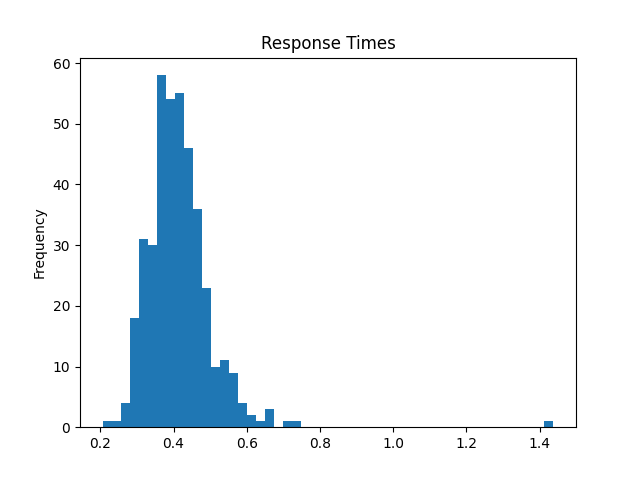
keep_first = "response"
metadata, events, event_id = mne.epochs.make_metadata(
    events=all_events,
    event_id=all_event_id,
    tmin=metadata_tmin,
    tmax=metadata_tmax,
    sfreq=raw.info["sfreq"],
    row_events=row_events,
    keep_first=keep_first,
)

# visualize response times regardless of side
metadata["response"].plot.hist(bins=50, title="Response Times (first response)")
The first_response column contains only "left" and "right" entries,
derived from the respective initial events "response/left" and
"response/right":
print(metadata["first_response"])
2       left
4       left
6      right
8       left
10      left
       ...
792     left
794    right
796     left
798    right
800     left
Name: first_response, Length: 400, dtype: object
For stimulus events, there are not only two, but four different types:
stimulus/compatible/target_left,
stimulus/compatible/target_right, stimulus/incompatible/target_left,
and stimulus/incompatible/target_right. What’s more, because in the
present paradigm stimuli were presented in rapid succession, sometimes
multiple stimulus events occurred within the 1.5 second time window we used
to generate our metadata. See for example:
metadata.loc[
    metadata["stimulus/compatible/target_left"].notna()
    & metadata["stimulus/compatible/target_right"].notna(),
    :,
]
Looking at the stimulus/compatible/target_left and
stimulus/compatible/target_right columns, you will see that both always contain a
numerical value (one is always zero, the other is not). This is because both events
occurred within the time window of 1.5 seconds.
This can easily lead to confusion during later stages of processing, so let’s
create a column for the first stimulus – which will always be the time-locked
stimulus, as our time interval starts at 0 seconds. We can pass a list of
strings to keep_first.
keep_first = ["stimulus", "response"]
metadata, events, event_id = mne.epochs.make_metadata(
    events=all_events,
    event_id=all_event_id,
    tmin=metadata_tmin,
    tmax=metadata_tmax,
    sfreq=raw.info["sfreq"],
    row_events=row_events,
    keep_first=keep_first,
)

# all times of the time-locked events should be zero
assert all(metadata["stimulus"] == 0)

# the values in the new "first_stimulus" and "first_response" columns indicate
# which events were selected via "keep_first"
metadata[["first_stimulus", "first_response"]]
Adding new columns to describe stimulation side and response correctness#
Perfect! Now it’s time to define which responses were correct and incorrect. We first add a column encoding the side of stimulation, and then simply check whether the response matches the stimulation side, and add this result to another column.
metadata.loc[:, "stimulus_side"] = ""  # initialize column

# left-side stimulation
metadata.loc[
    metadata["first_stimulus"].isin(
        ["compatible/target_left", "incompatible/target_left"]
    ),
    "stimulus_side",
] = "left"

# right-side stimulation
metadata.loc[
    metadata["first_stimulus"].isin(
        ["compatible/target_right", "incompatible/target_right"]
    ),
    "stimulus_side",
] = "right"

# first assume all responses were incorrect, then mark those as correct where
# the stimulation side matches the response side
metadata["response_correct"] = False
metadata.loc[
    metadata["stimulus_side"] == metadata["first_response"], "response_correct"
] = True

metadata
Count the number of correct and incorrect responses:
correct_response_count = metadata["response_correct"].sum()
print(
    f"Correct responses: {correct_response_count}\n"
    f"Incorrect responses: {len(metadata) - correct_response_count}"
)
Correct responses: 346
Incorrect responses: 54
Creating Epochs with metadata, and visualizing ERPs#
The metadata is ready. Now it’s finally time to create our epochs!
We will assign the metadata directly on epochs creation
via the metadata parameter. Also, it is important to
remember to pass the events and event_id that were returned from
make_metadata, as we only created metadata for a subset of
our original events by passing row_events. If we were to pass to “original”
values instead, the length of the metadata and the number of epochs would mismatch,
which would raise an error.
epochs_tmin, epochs_tmax = -0.1, 0.4  # epochs range: [-0.1, 0.4] s
reject = {"eeg": 250e-6}  # exclude epochs with strong artifacts
epochs = mne.Epochs(
    raw=raw,
    tmin=epochs_tmin,
    tmax=epochs_tmax,
    events=events,
    event_id=event_id,
    metadata=metadata,
    reject=reject,
    preload=True,
)
Adding metadata with 13 columns
400 matching events found
Setting baseline interval to [-0.099609375, 0.0] s
Applying baseline correction (mode: mean)
0 projection items activated
Using data from preloaded Raw for 400 events and 513 original time points ...
    Rejecting  epoch based on EEG : ['F8']
    Rejecting  epoch based on EEG : ['F8']
    Rejecting  epoch based on EEG : ['FP2']
    Rejecting  epoch based on EEG : ['FP2']
    Rejecting  epoch based on EEG : ['FP1', 'FP2']
    Rejecting  epoch based on EEG : ['FP1', 'FP2']
    Rejecting  epoch based on EEG : ['F8']
    Rejecting  epoch based on EEG : ['FP1', 'FP2']
    Rejecting  epoch based on EEG : ['F8']
9 bad epochs dropped
You probably also noticed that 9 epochs were dropped because they exceeded our rejection limits. This is another reason why it is important to assign the metadata on epochs creation: the metadata will be updated automatically to reflect the actual epochs that were kept.
Lastly, let’s visualize the ERPs associated with the visual stimulation. We will only consider trials with correct responses and produce three plots: one for all correct responses, one for correct slow responses (response time slower than 0.5 s), and one for correct fast responses (response time up to 0.5 s).
vis_erp = epochs["response_correct"].average()
vis_erp_slow = epochs["(response_correct) & (response > 0.5)"].average()
vis_erp_fast = epochs["(response_correct) & (response <= 0.5)"].average()

fig, ax = plt.subplots(3, figsize=(6, 8), layout="constrained")
vis_erp.plot(gfp=True, spatial_colors=True, axes=ax[0], show=False)
vis_erp_slow.plot(gfp=True, spatial_colors=True, axes=ax[1], show=False)
vis_erp_fast.plot(gfp=True, spatial_colors=True, axes=ax[2], show=False)

# Set titles
ax[0].set_title("All Correct Responses")
ax[1].set_title("Slow Correct Responses")
ax[2].set_title("Fast Correct Responses")
fig.suptitle("Visual ERPs", fontweight="bold")

# Turn of x axes for the first two plots
ax[0].xaxis.set_visible(False)
ax[1].xaxis.set_visible(False)
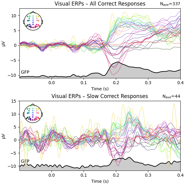
Aside from the fact that the data for the (much fewer) slow responses looks noisier – which is entirely to be expected – not much of an ERP difference can be seen.
Applying the knowledge: visualizing the ERN component#
In the following analysis, we will use the same dataset as above, but we’ll time-lock our epochs to the response events, not to the stimulus onset. Comparing ERPs associated with correct and incorrect behavioral responses, we should be able to see the error-related negativity (ERN) in the difference wave.
Since we want to time-lock our analysis to responses, for the automated metadata generation we’ll consider events occurring up to 1500 ms before the response trigger so we can be sure to capture the stimulation event as well.
We only wish to consider the last stimulus and response in each time
window: Remember that we’re dealing with rapid stimulus presentations in
this paradigm; taking the last response (time point zero) and the last
stimulus (the one closest to the response) ensures that we actually create
the right stimulus-response pairings. We can achieve this by passing the
keep_last parameter, which works exactly like keep_first we used
previously, only that it keeps the last occurrences of the specified
events and stores them in columns whose names start with last_.
metadata_tmin, metadata_tmax = -1.5, 0
row_events = ["response/left", "response/right"]
keep_last = ["stimulus", "response"]

metadata, events, event_id = mne.epochs.make_metadata(
    events=all_events,
    event_id=all_event_id,
    tmin=metadata_tmin,
    tmax=metadata_tmax,
    sfreq=raw.info["sfreq"],
    row_events=row_events,
    keep_last=keep_last,
)

metadata
Exactly like in the previous example, we create new columns stimulus_side
and response_correct.
metadata.loc[:, "stimulus_side"] = ""  # initialize column

# left-side stimulation
metadata.loc[
    metadata["last_stimulus"].isin(
        ["compatible/target_left", "incompatible/target_left"]
    ),
    "stimulus_side",
] = "left"

# right-side stimulation
metadata.loc[
    metadata["last_stimulus"].isin(
        ["compatible/target_right", "incompatible/target_right"]
    ),
    "stimulus_side",
] = "right"

# first assume all responses were incorrect, then mark those as correct where
# the stimulation side matches the response side
metadata["response_correct"] = False
metadata.loc[
    metadata["stimulus_side"] == metadata["last_response"], "response_correct"
] = True

metadata
Now it’s already time to epoch the data! When deciding upon the epochs duration for this specific analysis, we need to ensure to include quite a bit of signal from before and after the motor response. We also must be aware of the fact that motor-/muscle-related signals will most likely be present before the response button trigger pulse appears in our data, so the time period close to the response event should not be used for baseline correction. But at the same time, we don’t want to use a baseline period that extends too far away from the button event. The following values seem to work quite well. Remember: time point zero is the response event.
epochs_tmin, epochs_tmax = -0.6, 0.4
baseline = (-0.4, -0.2)
reject = {"eeg": 250e-6}
epochs = mne.Epochs(
    raw=raw,
    tmin=epochs_tmin,
    tmax=epochs_tmax,
    baseline=baseline,
    reject=reject,
    events=events,
    event_id=event_id,
    metadata=metadata,
    preload=True,
)
Adding metadata with 13 columns
402 matching events found
Applying baseline correction (mode: mean)
0 projection items activated
Using data from preloaded Raw for 402 events and 1025 original time points ...
    Rejecting  epoch based on EEG : ['F8']
    Rejecting  epoch based on EEG : ['FP1', 'F7', 'FP2']
    Rejecting  epoch based on EEG : ['F7', 'F8', 'FC4']
    Rejecting  epoch based on EEG : ['FC3', 'F4', 'FC4']
    Rejecting  epoch based on EEG : ['FP1']
    Rejecting  epoch based on EEG : ['FP2']
    Rejecting  epoch based on EEG : ['FP1', 'FP2']
    Rejecting  epoch based on EEG : ['FP2']
    Rejecting  epoch based on EEG : ['FP1', 'FP2']
    Rejecting  epoch based on EEG : ['FP1', 'FP2']
    Rejecting  epoch based on EEG : ['FP1', 'FP2']
    Rejecting  epoch based on EEG : ['FP1', 'FP2']
    Rejecting  epoch based on EEG : ['FP1', 'FP2']
    Rejecting  epoch based on EEG : ['FP2']
    Rejecting  epoch based on EEG : ['F8']
    Rejecting  epoch based on EEG : ['F8']
    Rejecting  epoch based on EEG : ['FP2', 'F8']
    Rejecting  epoch based on EEG : ['FP1', 'F3', 'F7', 'FC3', 'C3', 'C5', 'P3', 'CPz', 'Fz', 'F4', 'F8', 'FC4', 'FCz', 'Cz', 'C4', 'P4']
    Rejecting  epoch based on EEG : ['FP2']
    Rejecting  epoch based on EEG : ['FP2']
    Rejecting  epoch based on EEG : ['FP1', 'FP2', 'F8']
    Rejecting  epoch based on EEG : ['FP2']
    Rejecting  epoch based on EEG : ['FP1', 'FP2']
    Rejecting  epoch based on EEG : ['FP1', 'FP2']
    Rejecting  epoch based on EEG : ['FP2']
    Rejecting  epoch based on EEG : ['FP1', 'FP2']
    Rejecting  epoch based on EEG : ['FP2']
    Rejecting  epoch based on EEG : ['FP2']
    Rejecting  epoch based on EEG : ['FP2']
    Rejecting  epoch based on EEG : ['FP2']
    Rejecting  epoch based on EEG : ['FP1', 'FP2']
    Rejecting  epoch based on EEG : ['FP1', 'FP2']
    Rejecting  epoch based on EEG : ['FP2']
    Rejecting  epoch based on EEG : ['FP2']
    Rejecting  epoch based on EEG : ['FP2', 'F8']
    Rejecting  epoch based on EEG : ['F8']
36 bad epochs dropped
Let’s do a final sanity check: we want to make sure that in every row, we
actually have a stimulus. We use epochs.metadata (and not metadata)
because when creating the epochs, we passed the reject parameter, and
MNE-Python always ensures that epochs.metadata stays in sync with the
available epochs. During epochs creation, several epochs were dropped as they
exceeded the rejection limits.
epochs.metadata.loc[epochs.metadata["last_stimulus"].isna(), :]
Bummer! It seems the very first two responses were recorded before the
first stimulus appeared: the values in the stimulus column are None.
There is a very simple way to select only those epochs that do have a
stimulus (i.e., are not None):
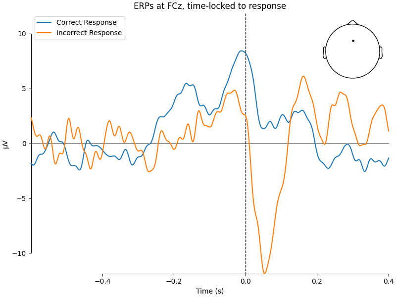
Now it’s time to calculate the ERPs for correct and incorrect responses.
For visualization, we’ll only look at sensor FCz, which is known to show
the ERN nicely in the given paradigm.
resp_erp_correct = epochs["response_correct"].average()
resp_erp_incorrect = epochs["not response_correct"].average()

mne.viz.plot_compare_evokeds(
    {"Correct Response": resp_erp_correct, "Incorrect Response": resp_erp_incorrect},
    picks="FCz",
    show_sensors=True,
    title="ERPs at FCz, time-locked to response",
)
We’ll also create a topoplot to get an impression of the average scalp potentials measured in the first 100 ms after an incorrect response.
# topoplot of average field from time 0.0-0.1 s
fig = resp_erp_incorrect.plot_topomap(times=0.05, average=0.1, size=3)
fig.suptitle("Mean topography after incorrect responses", fontsize=14)
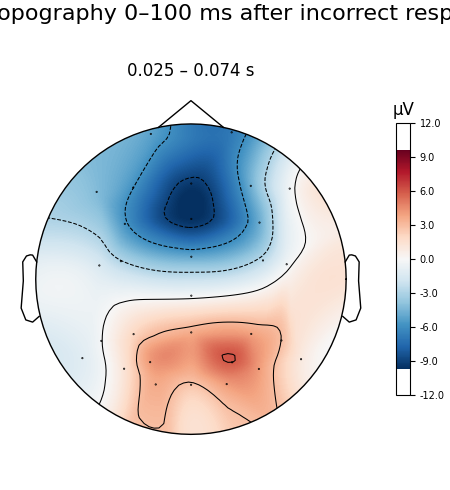
We can see a strong negative deflection immediately after incorrect responses, compared to correct responses. The topoplot, too, leaves no doubt: what we’re looking at is, in fact, the ERN.
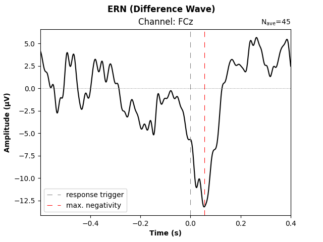
Some researchers suggest to construct the difference wave between ERPs for correct and incorrect responses, as it more clearly reveals signal differences, while ideally also improving the signal-to-noise ratio (under the assumption that the noise level in “correct” and “incorrect” trials is similar). Let’s do just that and put it into a publication-ready visualization.
# difference wave: incorrect minus correct responses
resp_erp_diff = mne.combine_evoked(
    [resp_erp_incorrect, resp_erp_correct], weights=[1, -1]
)

fig, ax = plt.subplots()
resp_erp_diff.plot(picks="FCz", axes=ax, selectable=False, show=False)

# make ERP trace bolder
ax.lines[0].set_linewidth(1.5)

# add lines through origin
ax.axhline(0, ls="dotted", lw=0.75, color="gray")
ax.axvline(0, ls=(0, (10, 10)), lw=0.75, color="gray", label="response trigger")

# mark trough
trough_time_idx = resp_erp_diff.copy().pick("FCz").data.argmin()
trough_time = resp_erp_diff.times[trough_time_idx]
ax.axvline(trough_time, ls=(0, (10, 10)), lw=0.75, color="red", label="max. negativity")

# legend, axis labels, title
ax.legend(loc="lower left")
ax.set_xlabel("Time (s)", fontweight="bold")
ax.set_ylabel("Amplitude (µV)", fontweight="bold")
ax.set_title("Channel: FCz")
fig.suptitle("ERN (Difference Wave)", fontweight="bold")
References#
Total running time of the script: (0 minutes 22.717 seconds)