Generate simulated source data

This example illustrates how to use the mne.simulation.SourceSimulator class to generate source estimates and raw data. It is meant to be a brief introduction and only highlights the simplest use case.

# Author: Kostiantyn Maksymenko <kostiantyn.maksymenko@gmail.com>
#         Samuel Deslauriers-Gauthier <sam.deslauriers@gmail.com>
#
# License: BSD-3-Clause
# Copyright the MNE-Python contributors.

import numpy as np

import mne
from mne.datasets import sample

print(__doc__)

For this example, we will be using the information of the sample subject. This will download the data if it not already on your machine. We also set the subjects directory so we don’t need to give it to functions.

data_path = sample.data_path()
subjects_dir = data_path / "subjects"
subject = "sample"

First, we get an info structure from the test subject.

evoked_fname = data_path / "MEG" / subject / "sample_audvis-ave.fif"
info = mne.io.read_info(evoked_fname)
tstep = 1.0 / info["sfreq"]

Read a total of 4 projection items:
    PCA-v1 (1 x 102) active
    PCA-v2 (1 x 102) active
    PCA-v3 (1 x 102) active
    Average EEG reference (1 x 60) active

To simulate sources, we also need a source space. It can be obtained from the forward solution of the sample subject.

fwd_fname = data_path / "MEG" / subject / "sample_audvis-meg-eeg-oct-6-fwd.fif"
fwd = mne.read_forward_solution(fwd_fname)
src = fwd["src"]

Reading forward solution from /home/circleci/mne_data/MNE-sample-data/MEG/sample/sample_audvis-meg-eeg-oct-6-fwd.fif...
    Reading a source space...
    Computing patch statistics...
    Patch information added...
    Distance information added...
    [done]
    Reading a source space...
    Computing patch statistics...
    Patch information added...
    Distance information added...
    [done]
    2 source spaces read
    Desired named matrix (kind = 3523) not available
    Read MEG forward solution (7498 sources, 306 channels, free orientations)
    Desired named matrix (kind = 3523) not available
    Read EEG forward solution (7498 sources, 60 channels, free orientations)
    Forward solutions combined: MEG, EEG
    Source spaces transformed to the forward solution coordinate frame

To select a region to activate, we use the caudal middle frontal to grow a region of interest.

selected_label = mne.read_labels_from_annot(
    subject, regexp="caudalmiddlefrontal-lh", subjects_dir=subjects_dir
)[0]
location = "center"  # Use the center of the region as a seed.
extent = 10.0  # Extent in mm of the region.
label = mne.label.select_sources(
    subject, selected_label, location=location, extent=extent, subjects_dir=subjects_dir
)

Reading labels from parcellation...
   read 1 labels from /home/circleci/mne_data/MNE-sample-data/subjects/sample/label/lh.aparc.annot
   read 0 labels from /home/circleci/mne_data/MNE-sample-data/subjects/sample/label/rh.aparc.annot

Define the time course of the activity for each source of the region to activate. Here we use a sine wave at 18 Hz with a peak amplitude of 10 nAm.

source_time_series = np.sin(2.0 * np.pi * 18.0 * np.arange(100) * tstep) * 10e-9

Define when the activity occurs using events. The first column is the sample of the event, the second is not used, and the third is the event id. Here the events occur every 200 samples.

n_events = 50
events = np.zeros((n_events, 3), int)
events[:, 0] = 100 + 200 * np.arange(n_events)  # Events sample.
events[:, 2] = 1  # All events have the sample id.

Create simulated source activity. Here we use a SourceSimulator whose add_data method is key. It specified where (label), what (source_time_series), and when (events) an event type will occur.

source_simulator = mne.simulation.SourceSimulator(src, tstep=tstep)
source_simulator.add_data(label, source_time_series, events)

Project the source time series to sensor space and add some noise. The source simulator can be given directly to the simulate_raw function.

raw = mne.simulation.simulate_raw(info, source_simulator, forward=fwd)
cov = mne.make_ad_hoc_cov(raw.info)
mne.simulation.add_noise(raw, cov, iir_filter=[0.2, -0.2, 0.04])
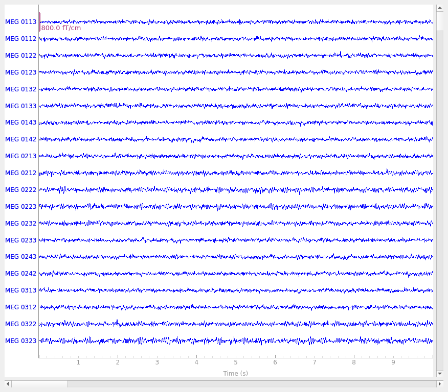
raw.plot()

Setting up raw simulation: 1 position, "cos2" interpolation
Event information stored on channel:              STI 014
    Interval 0.000–1.665 s
Setting up forward solutions
Computing gain matrix for transform #1/1
    Interval 0.000–1.665 s
    Interval 0.000–1.665 s
    Interval 0.000–1.665 s
    Interval 0.000–1.665 s
    Interval 0.000–1.665 s
    Interval 0.000–1.665 s
    Interval 0.000–1.665 s
    Interval 0.000–1.665 s
    Interval 0.000–1.665 s
    10 STC iterations provided
[done]
Adding noise to 366/376 channels (366 channels in cov)

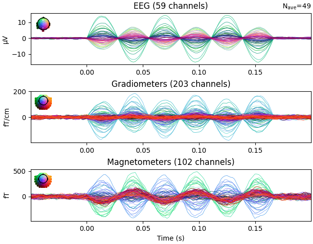
Plot evoked data to get another view of the simulated raw data.

events = mne.find_events(raw)
epochs = mne.Epochs(raw, events, 1, tmin=-0.05, tmax=0.2)
evoked = epochs.average()
evoked.plot()

50 events found on stim channel STI 014
Event IDs: [1]
Not setting metadata
50 matching events found
Setting baseline interval to [-0.049948803289596964, 0.0] s
Applying baseline correction (mode: mean)
Created an SSP operator (subspace dimension = 4)
4 projection items activated

Estimated memory usage: 211 MB